One of the key techniques of exploratory data mining is clustering – separating instances into distinct groups based on some measure of similarity. [1] In this post we will review how we can do clustering, evaluate and visualize results using online ML Sandbox tool from this website. This tool allows to run some machine learning algorithms without coding and setup/install. The following components will be explored:
Clustering Algorithms
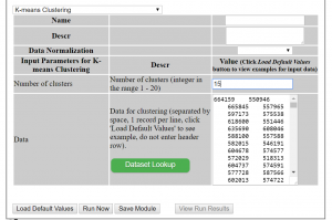
K-means Clustering Algorithm – is well known algorithm as the idea of this algorithm goes back to 1957. [2] The algorithm requires to input number of clusters and data. k-means clustering aims to partition n observations into k clusters in which each observation belongs to the cluster with the nearest mean.[2]. Below are shown results of K-means clustering of Iris dataset (only 2 dimensions shown) and clustering result for S1 dataset (see dataset section for more details).
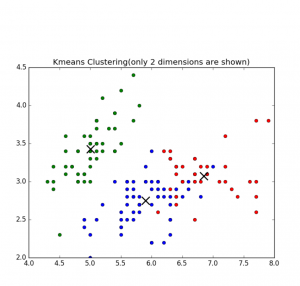
Fig 1. K-means clustering of Iris dataset
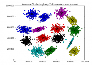
Fig 2. K-means clustering of S1 dataset
Affinity Propagation – performs affinity propagation clustering of data. In statistics and data mining, affinity propagation (AP) is a clustering algorithm based on the concept of “message passing” between data points. Unlike clustering algorithms such as k-means or k-medoids, affinity propagation does not require the number of clusters to be determined or estimated before running the algorithm. Similar to k-medoids, affinity propagation finds “exemplars”, members of the input set that are representative of clusters.[3]
Hierarchical clustering (HC) – (also called hierarchical cluster analysis or HCA) is a method of cluster analysis which seeks to build a hierarchy of clusters. Strategies for hierarchical clustering generally fall into two types:
- Agglomerative: This is a “bottom up” approach: each observation starts in its own cluster, and pairs of clusters are merged as one moves up the hierarchy.
- Divisive: This is a “top down” approach: all observations start in one cluster, and splits are performed recursively as one moves down the hierarchy.
In general, the merges and splits are determined in a greedy manner. The results of hierarchical clustering are usually presented in a dendrogram. [4]
Birch algorithm – Back in the 1990s considerable effort has been put into improving the performance of existing algorithms. Among them is BIRCH (Zhang et al., 1996) [5]
BIRCH (balanced iterative reducing and clustering using hierarchies) is an unsupervised data mining algorithm used to perform hierarchical clustering over particularly large data-sets. An advantage of BIRCH is its ability to incrementally and dynamically cluster incoming, multi-dimensional metric data points in an attempt to produce the best quality clustering for a given set of resources (memory and time constraints). In most cases, BIRCH only requires a single scan of the database. [6]
Performance metrics for clustering algorithms
Silhouette refers to a method of interpretation and validation of consistency within clusters of data. The technique provides a succinct graphical representation of how well each object lies within its cluster. It was first described by Peter J. Rousseeuw in 1986.
The silhouette value is a measure of how similar an object is to its own cluster (cohesion) compared to other clusters (separation). The silhouette ranges from -1 to 1, where a high value indicates that the object is well matched to its own cluster and poorly matched to neighboring clusters. If most objects have a high value, then the clustering configuration is appropriate. If many points have a low or negative value, then the clustering configuration may have too many or too few clusters.
The silhouette can be calculated with any distance metric, such as the Euclidean distance or the Manhattan distance.[7]
Here is the python source code how to calculate the silhouette value for k-means clustering
from sklearn import cluster
from sklearn import metrics
import numpy as np


k=2
data = np.array([[1, 2],
              [5, 8],
              [1.5, 1.8],
              [8, 8],
              [1, 0.6],
              [9, 11]])


kmeans = cluster.KMeans(n_clusters=k)
kmeans.fit(data)


labels = kmeans.labels_
centroids = kmeans.cluster_centers_

print ("Cluster id labels for inputted data")
print (labels)
print ("Centroids data")
print (centroids)

print ("\nScore (Opposite of the value of X on the K-means objective which is Sum of distances of samples to their closest cluster center):")
print (kmeans.score(data))

silhouette_score = metrics.silhouette_score(data, labels, metric='euclidean')

print ("Silhouette_score: ")
print (silhouette_score)
Score (Opposite of the value of X on the K-means objective which is Sum of distances of samples to their closest cluster center) – Sum of distances of samples to their closest cluster center.
Large distances corresponds to a big variety in data samples and if the number of data samples is significantly higher than the number of clusters. On the contrary, if all data samples were the same, you would always get a zero distance regardless of number of clusters. [8]
Cophenetic correlation – In statistics, and especially in biostatistics, cophenetic correlation (more precisely, the cophenetic correlation coefficient) is a measure of how faithfully a dendrogram preserves the pairwise distances between the original unmodeled data points. Although it has been most widely applied in the field of biostatistics (typically to assess cluster-based models of DNA sequences, or other taxonomic models), it can also be used in other fields of inquiry where raw data tend to occur in clumps, or clusters. This coefficient has also been proposed for use as a test for nested clusters.[9]
Datasets
The following two datasets will be used:
The Iris flower data set or Fisher’s Iris data set is a multivariate data set – well know data set with N = 150 and k=3 [10] The data set consists of 50 samples from each of three species of Iris (Iris setosa, Iris virginica and Iris versicolor) [10]
S1 – Synthetic 2-d data with N=5000 vectors and k=15 Gaussian cluster [11]
Experiments
Using ML Sandbox tool and above clustering algorithms and datasets the clustering was performed. Screenshots of results of clustering from the tool were collected and presented here (Fig 1-6, Fig 1,2 are shown above)
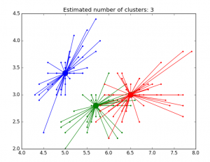
Fig 3. AP clustering of Iris dataset
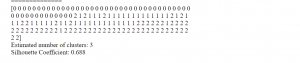
Fig 4. AP clustering results of Iris dataset
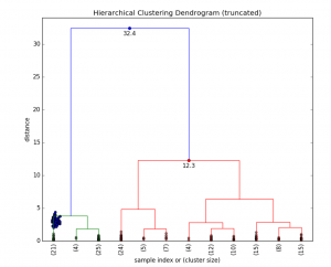
Fig 5. HC Clustering Iris dataset
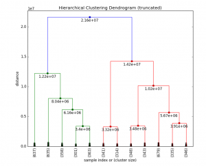
Fig 6. HC clustering S1 dataset
Below in the summary of the above clustering experiments.
| Kmeans (sklearn.cluster) | AP (sklearn.cluster) | HC (scipy.cluster) | Birch (sklearn.cluster) | ||
| Score (Opposite of Sum of distances of samples to their closest cluster center) | Silhouette_score | Silhouette_score | Cophenetic Correlation Coefficient: | Silhouette_score | |
| Iris dataset, 150, D4 | -78.85 | 0.55 | 0.52 | 0.87 | 0.50 |
| S1 dataset, 5000, D2 | -8.92e+12 | 0.71 | * | 0.69 | 0.71 |
*AP did not work well on S1 dataset (but worked well on iris dataset) however there are some other optional parameters that can be used to resolve this. Probably need to be adjust preference parameter. Currently the tool does not allow change it.
From documentation [12] Preference is parameter that can be array-like, shape (n_samples,) or float, and is optional. Preferences for each point – points with larger values of preferences are more likely to be chosen as exemplars. The number of exemplars, ie of clusters, is influenced by the input preferences value. If the preferences are not passed as arguments, they will be set to the median of the input similarities.
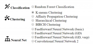
ML Sandbox
The above tool was used for clustering data. You need just select algorithm, enter your data and click run. Below are detailed instructions for clustering.
How to use the ML Sandbox
1. Open URL: ML Sandbox
2. Select Clustering method
3. Enter data (you can use default small dataset or copy and paste your dataset or dataset from other sites like iris, S1 see links in the references section)
4. Click Run Now
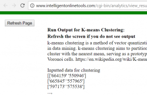
5. Click View Run Results
6. If you do not see results, click refresh button at top left corner. Depending on data set and algorithm you might need wait for a minute or two and click refresh.
Conclusion
We looked at different clustering methods, metrics performance and visualization of clustering results for different datasets. All of this can be done within online tool ML Sandbox Feel free to play with this tool and your data to explore your datasets. Also feel free to provide any feedback or suggestions.
References
1. Hierarchical Clustering: A Simple Explanation
2. k-means clustering
3. Affinity_propagation
4. Hierarchical clustering
5. Cluster_analysis
6. BIRCH
7. Silhouette (clustering)
8. understanding-score-returned-by-scikit-learn-kmeans
9. Cophenetic correlation
10. Iris flower data set
11. Clustering benchmark datasets
12 AffinityPropagation