Applied Machine Learning Classification for Decision Making

Making the good decision is the challenge that we often have. So, in this post, we will look at how applied machine learning classification can be used for the process of decision making.

The simple and quick approach to make decision is follow our past experience of similar situations. Usually we use compiling a list of pros and cons, asking someone for help or searching on the web. According to [1] we have two systems in our brain: logical and intuitive system:

“With every decision you take, every judgement you make, there is a battle in your mind – a battle between intuition and logic.”

“Most of the beliefs or opinions you have come from an automatic response. But then your logical mind invents a reason why you think or believe something.”

Most of the time our intuitive system is working efficiently, taking charge of all the thousands of decisions we make each day. But our intuitive system can be biased in many ways. For example it can be biased toward the latest unsuccessful outcome.

Besides this our memory can not remember a lot of information so we can not use efficiently all our past information and experience. That’s why people created tools like decision matrix that can help to improve decision making. In the next section we will look at techniques that facilitates using our rational decision making.

Decision Making

Decision Matrix

More advanced approach for making decision is score each possible option. In this approach we score each option against some criteria or feature. For example for the candidate product that we need to buy we are looking at price, quality, service and safety features. This approach results in creating decision matrix for analysis of possible options.

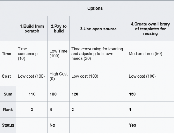
Below is an example of decision matrix [3] for choosing strategy for building some software project. Here we score 4 options based on the time to build and cost. The score is on the scale 0 (worst) – 100 (best). After we score each cell for time and cost rows, we can get sum of scores, rank and then make our choice (see last 3 rows)

Decision Matrix Example

There are also other, similar to decision matrix tools: belief decision matrix[3], Pugh Matrix[4].
These tools allow do comparison analysis of available options vs features and this enforces our mind logically evaluate and rank as much as possible pros and cons based on some numerical metrics.

However there are some limitations also. Incorrect selection criteria will obviously lead to the wrong conclusion. Poorly defined criteria can have multiple interpretations. For example too low can mean different things. With many rows or columns it becomes labor intensive to fill out the matrix.

Machine Learning Approach for Making Decision

Machine learning techniques can also help us improve decision making and even solve some of the above limitations. For example with Feature Engineering we can evaluate what criteria are important for decision.

In machine learning making decision can be viewed as assigning or predicting correct label (for example buy, not buy) based on data for the item features. In the field of machine learning or AI this is known as classification problem.

Classification algorithms learn correct decisions from data. Below is the example of training data that we input to machine learning classification algorithm. (Xij represent some numerical values)

Classification problem

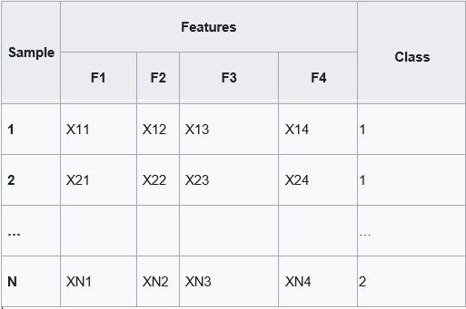
Our options (decisions) are now represented by class label (most right column), criteria are represented by features. So we now switched columns with rows. Using training data like above we train classifier and then use it to choose the class (make decision) for new data.

There are different classification algorithms such as decision tree, SVM, Naive Bayes, neural network classification. In this post we will look at classification with neural network.
We will use Keras neural network with 2 dense layers.

Per Keras documentation[5] Dense layer implements the operation:
output = activation(dot(input, kernel) + bias)
where activation is the element-wise activation function passed as the activation argument,
kernel is a weights matrix created by the layer,
and bias is a bias vector created by the layer (only applicable if use_bias is True).

So we can see that the dense layer is performing similar math that we were doing in decision matrix.

Python Source Code for Neural Network Classification Algorithms

Finally, below is the python source code for classification problem. To test this code we will use iris dataset. This dataset has 3 classes and 4 features. Our task here to make the classifier able to assign correct label class.

# -*- coding: utf-8 -*-

from keras.utils import to_categorical
from sklearn import datasets

iris = datasets.load_iris()

# Create feature matrix
X = iris.data
print (X)

# Create target vector
y = iris.target
y = to_categorical(y, num_classes=3)
print (y)

from sklearn.model_selection import train_test_split

x_train, x_test, y_train, y_test = train_test_split( X, y, test_size=0.33, random_state=42)

print (x_train)
print (y_train)

from keras.models import Sequential
from keras.layers import Dense

model = Sequential()
model.add(Dense(32, input_shape=(4,), activation='relu',  name='L1'))
model.add(Dense(3, activation='softmax', name='L2'))
model.compile(optimizer='rmsprop',
              loss='categorical_crossentropy',
              metrics=['accuracy'])

print('Model Summary:')
print(model.summary())

model.fit(x_train, y_train, verbose=2, batch_size=10, epochs=100)
output = model.evaluate(x_test, y_test)

print('Final test loss: {:4f}'.format(output[0]))
print('Final test accuracy: {:4f}'.format(output[1]))


Below are results of neural network run.

Results of neural network run

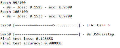
As we can see our classifier is able to make correct decisions with 98% accuracy.

Thus we investigated different approaches for making decision. We saw how machine learning can be applied to this too. Specifically we looked at neural network classification algorithm for selecting correct label.
I would love to hear what types of decision making tools do you use for making decisions? Also feel free to provide feedback or suggestions.

References
1. How do we really make decisions?
2. What Is a Decision Matrix? Definition and Examples
3. Decision matrix From Wikipedia, the free encyclopedia
4. The Systems Engineering Tool Box
5. Keras Documentation


LSTM Neural Network Training – Few Useful Techniques for Tuning Hyperparameters and Saving Time

Neural networks are among the most widely used machine learning techniques.[1] But neural network training and tuning multiple hyper-parameters takes time. I was recently building LSTM neural network for prediction for this post Machine Learning Stock Market Prediction with LSTM Keras and I learned some tricks that can save time. In this post you will find some techniques that helped me to do neural net training more efficiently.

1. Adjusting Graph To See All Details

Sometimes validation loss is getting high value and this prevents from seeing other data on the chart. I added few lines of code to cut high values so you can see all details on chart.

import matplotlib.pyplot as plt
import matplotlib.ticker as mtick

T=25
history_val_loss=[]

for x in history.history['val_loss']:
      if x >= T:
             history_val_loss.append (T)
      else:
             history_val_loss.append( x )

plt.figure(6)
plt.plot(history.history['loss'])
plt.plot(history_val_loss)
plt.title('model loss adjusted')
plt.ylabel('loss')
plt.xlabel('epoch')
plt.legend(['train', 'test'], loc='upper left')

Below is the example of charts. Left graph is not showing any details except high value point because of the scale. Note that graphs are obtained from different tests.

LSTM NN Training Value Loss Charts with High Number and Adjusted

2. Early Stopping

Early stopping is allowing to save time on not running tests when a monitored quantity has stopped improving. Here is how it can be coded:

earlystop = EarlyStopping(monitor='val_loss', min_delta=0.0001, patience=80,  verbose=1, mode='min')
callbacks_list = [earlystop]

history=model.fit (x_train, y_train, batch_size =1, nb_epoch =1000, shuffle = False, validation_split=0.15, callbacks=callbacks_list)

Here is what arguments mean per Keras documentation [2].

min_delta: minimum change in the monitored quantity to qualify as an improvement, i.e. an absolute change of less than min_delta, will count as no improvement.
patience: number of epochs with no improvement after which training will be stopped.
verbose: verbosity mode.
mode: one of {auto, min, max}. In min mode, training will stop when the quantity monitored has stopped decreasing; in max mode it will stop when the quantity monitored has stopped increasing; in auto mode, the direction is automatically inferred from the name of the monitored quantity.

3. Weight Regularization

Weight regularizer can be used to regularize neural net weights. Here is the example.

from keras.regularizers import L1L2
model.add (LSTM ( 400,  activation = 'relu', inner_activation = 'hard_sigmoid' , bias_regularizer=L1L2(l1=0.01, l2=0.01),  input_shape =(len(cols), 1), return_sequences = False ))

Below are the charts that are showing impact of weight regularizer on loss value :

LSTM NN Training Value Loss without weigh regularization

LSTM NN Training Value Loss without weigh regularization

Without weight regularization validation loss is going more up during the neural net training.

4. Optimizer

Keras software allows to use different optimizers. I was using adam optimizer which is widely used. Here is how it can be used:

adam=optimizers.Adam(lr=0.01, beta_1=0.91, beta_2=0.999, epsilon=None, decay=0.0, amsgrad=True)
model.compile (loss ="mean_squared_error" , optimizer = "adam") 

I found that beta_1=0.89 performed better then suggested 0.91 or other tested values.

5. Rolling Window Size

Rolling window (in case we use it) also can impact on performance. Too small or too big will drive higher validation loss. Below are charts for different window size (N=4,8,16,18, from left to right). In this case the optimal value was 16 which resulted in 81% accuracy.

LSTM Neural Net Loss Charts with Different N

I hope you enjoyed this post on different techniques for tuning hyper parameters. If you have any tips or anything else to add, please leave a comment below in the comment box.

Below is the full source code:

import numpy as np
import pandas as pd
from sklearn import preprocessing

import matplotlib.pyplot as plt
import matplotlib.ticker as mtick

from keras.regularizers import L1L2

fname="C:\\Users\\stock data\\GM.csv"
data_csv = pd.read_csv (fname)

#how many data we will use 
# (should not be more than dataset length )
data_to_use= 150

# number of training data
# should be less than data_to_use
train_end =120


total_data=len(data_csv)

#most recent data is in the end 
#so need offset
start=total_data - data_to_use


yt = data_csv.iloc [start:total_data ,4]    #Close price
yt_ = yt.shift (-1)   

print (yt_)

data = pd.concat ([yt, yt_], axis =1)
data. columns = ['yt', 'yt_']


N=16    
cols =['yt']
for i in range (N):
  
    data['yt'+str(i)] = list(yt.shift(i+1))
    cols.append ('yt'+str(i))
    
data = data.dropna()
data_original = data
data=data.diff()
data = data.dropna()
    
    
# target variable - closed price
# after shifting
y = data ['yt_']
x = data [cols]

   
scaler_x = preprocessing.MinMaxScaler ( feature_range =( -1, 1))
x = np. array (x).reshape ((len( x) ,len(cols)))
x = scaler_x.fit_transform (x)

scaler_y = preprocessing. MinMaxScaler ( feature_range =( -1, 1))
y = np.array (y).reshape ((len( y), 1))
y = scaler_y.fit_transform (y)

    
x_train = x [0: train_end,]
x_test = x[ train_end +1:len(x),]    
y_train = y [0: train_end] 
y_test = y[ train_end +1:len(y)]  

x_train = x_train.reshape (x_train. shape + (1,)) 
x_test = x_test.reshape (x_test. shape + (1,))

from keras.models import Sequential
from keras.layers.core import Dense
from keras.layers.recurrent import LSTM
from keras.layers import  Dropout
from keras import optimizers

from numpy.random import seed
seed(1)
from tensorflow import set_random_seed
set_random_seed(2)

from keras import regularizers

from keras.callbacks import EarlyStopping


earlystop = EarlyStopping(monitor='val_loss', min_delta=0.0001, patience=80,  verbose=1, mode='min')
callbacks_list = [earlystop]

model = Sequential ()
model.add (LSTM ( 400,  activation = 'relu', inner_activation = 'hard_sigmoid' , bias_regularizer=L1L2(l1=0.01, l2=0.01),  input_shape =(len(cols), 1), return_sequences = False ))
model.add(Dropout(0.3))
model.add (Dense (output_dim =1, activation = 'linear', activity_regularizer=regularizers.l1(0.01)))
adam=optimizers.Adam(lr=0.01, beta_1=0.89, beta_2=0.999, epsilon=None, decay=0.0, amsgrad=True)
model.compile (loss ="mean_squared_error" , optimizer = "adam") 
history=model.fit (x_train, y_train, batch_size =1, nb_epoch =1000, shuffle = False, validation_split=0.15, callbacks=callbacks_list)


y_train_back=scaler_y.inverse_transform (np. array (y_train). reshape ((len( y_train), 1)))
plt.figure(1)
plt.plot (y_train_back)


fmt = '%.1f'
tick = mtick.FormatStrFormatter(fmt)
ax = plt.axes()
ax.yaxis.set_major_formatter(tick)
print (model.summary())

print(history.history.keys())

T=25
history_val_loss=[]

for x in history.history['val_loss']:
      if x >= T:
             history_val_loss.append (T)
      else:
             history_val_loss.append( x )


plt.figure(2)
plt.plot(history.history['loss'])
plt.plot(history.history['val_loss'])
plt.title('model loss')
plt.ylabel('loss')
plt.xlabel('epoch')
plt.legend(['train', 'test'], loc='upper left')
fmt = '%.1f'
tick = mtick.FormatStrFormatter(fmt)
ax = plt.axes()
ax.yaxis.set_major_formatter(tick)


plt.figure(6)
plt.plot(history.history['loss'])
plt.plot(history_val_loss)
plt.title('model loss adjusted')
plt.ylabel('loss')
plt.xlabel('epoch')
plt.legend(['train', 'test'], loc='upper left')


score_train = model.evaluate (x_train, y_train, batch_size =1)
score_test = model.evaluate (x_test, y_test, batch_size =1)
print (" in train MSE = ", round( score_train ,4)) 
print (" in test MSE = ", score_test )

pred1 = model.predict (x_test) 
pred1 = scaler_y.inverse_transform (np. array (pred1). reshape ((len( pred1), 1)))
 
prediction_data = pred1[-1]     
model.summary()
print ("Inputs: {}".format(model.input_shape))
print ("Outputs: {}".format(model.output_shape))
print ("Actual input: {}".format(x_test.shape))
print ("Actual output: {}".format(y_test.shape))

print ("prediction data:")
print (prediction_data)

y_test = scaler_y.inverse_transform (np. array (y_test). reshape ((len( y_test), 1)))
print ("y_test:")
print (y_test)

act_data = np.array([row[0] for row in y_test])

fmt = '%.1f'
tick = mtick.FormatStrFormatter(fmt)
ax = plt.axes()
ax.yaxis.set_major_formatter(tick)

plt.figure(3)
plt.plot( y_test, label="actual")
plt.plot(pred1, label="predictions")

print ("act_data:")
print (act_data)

print ("pred1:")
print (pred1)

plt.legend(loc='upper center', bbox_to_anchor=(0.5, -0.05),
          fancybox=True, shadow=True, ncol=2)


fmt = '$%.1f'
tick = mtick.FormatStrFormatter(fmt)
ax = plt.axes()
ax.yaxis.set_major_formatter(tick)

def moving_test_window_preds(n_future_preds):

    ''' n_future_preds - Represents the number of future predictions we want to make
                         This coincides with the number of windows that we will move forward
                         on the test data
    '''
    preds_moving = []                                    # Store the prediction made on each test window
    moving_test_window = [x_test[0,:].tolist()]          # First test window
    moving_test_window = np.array(moving_test_window)    
   
    for i in range(n_future_preds):
      
      
        preds_one_step = model.predict(moving_test_window) 
        preds_moving.append(preds_one_step[0,0]) 
                       
        preds_one_step = preds_one_step.reshape(1,1,1) 
        moving_test_window = np.concatenate((moving_test_window[:,1:,:], preds_one_step), axis=1) # new moving test window, where the first element from the window has been removed and the prediction  has been appended to the end
        

    print ("pred moving before scaling:")
    print (preds_moving)
                                         
    preds_moving = scaler_y.inverse_transform((np.array(preds_moving)).reshape(-1, 1))
    
    print ("pred moving after scaling:")
    print (preds_moving)
    return preds_moving
    
print ("do moving test predictions for next 22 days:")    
preds_moving = moving_test_window_preds(22)


count_correct=0
error =0
for i in range (len(y_test)):
    error=error + ((y_test[i]-preds_moving[i])**2) / y_test[i]

 
    if y_test[i] >=0 and preds_moving[i] >=0 :
        count_correct=count_correct+1
    if y_test[i] < 0 and preds_moving[i] < 0 :
        count_correct=count_correct+1

accuracy_in_change =  count_correct / (len(y_test) )

plt.figure(4)
plt.title("Forecast vs Actual, (data is differenced)")          
plt.plot(preds_moving, label="predictions")
plt.plot(y_test, label="actual")
plt.legend(loc='upper center', bbox_to_anchor=(0.5, -0.05),
          fancybox=True, shadow=True, ncol=2)


print ("accuracy_in_change:")
print (accuracy_in_change)

ind=data_original.index.values[0] + data_original.shape[0] -len(y_test)-1
prev_starting_price = data_original.loc[ind,"yt_"]
preds_moving_before_diff =  [0 for x in range(len(preds_moving))]

for i in range (len(preds_moving)):
    if (i==0):
        preds_moving_before_diff[i]=prev_starting_price + preds_moving[i]
    else:
        preds_moving_before_diff[i]=preds_moving_before_diff[i-1]+preds_moving[i]


y_test_before_diff = [0 for x in range(len(y_test))]

for i in range (len(y_test)):
    if (i==0):
        y_test_before_diff[i]=prev_starting_price + y_test[i]
    else:
        y_test_before_diff[i]=y_test_before_diff[i-1]+y_test[i]


plt.figure(5)
plt.title("Forecast vs Actual (non differenced data)")
plt.plot(preds_moving_before_diff, label="predictions")
plt.plot(y_test_before_diff, label="actual")
plt.legend(loc='upper center', bbox_to_anchor=(0.5, -0.05),
          fancybox=True, shadow=True, ncol=2)
plt.show()

References
1. Enhancing Neural Network Models for Knowledge Base Completion
2. Usage of callbacks
3. Rolling Window Regression: a Simple Approach for Time Series Next value Predictions


Machine Learning Stock Market Prediction with LSTM Keras

In the previous posts [1,2] I created script for machine learning stock market price on next day prediction. But it was pointed by readers that in stock market prediction, it is more important to know the trend: will the stock go up or down. So I updated the script to predict difference between today and yesterday prices. If it is negative the stock price will go down, if positive it will go up. Below will be described implemented modifications.

Data inputting

Data from previous days are entered as features through additional columns. The number of columns can be changed through parameter N in the beginning of script. So for example for day 20 the input will contain data for day 21 as target and data for days 20, 19,18,17… 20-N
Also added differencing before scaling. Differencing helped to improve performance of network. It also makes easy to get changes from previous day. In the end the differenced data inverted back.

Below is the stock data prices after applying differencing (subtructing previous day stock data price from current day)

Stock Data Prices after Differencing

Predicting future changes

I used moving_test_window_preds function. Inside of this function the script within loop is adding new prediction to “moving window” array and removing first element from it. This is based on example from blog post on forecasting time series with LSTM[4].
So the script is predicting future day data based on the previous known data in the “moving window”, updating known data and starting again. The performance evaluated by comparing predicted data with test (not used before) data.

LSTM Configuration

The LSTM network is constructed as following:

model = Sequential ()
input_shape =(len(cols), 1) ))
model.add (LSTM ( 400,  activation = 'relu', inner_activation = 'hard_sigmoid' , bias_regularizer=L1L2(l1=0.01, l2=0.01),  input_shape =(len(cols), 1), return_sequences = False ))
model.add(Dropout(0.3))
from keras import optimizers
model.add (Dense (output_dim =1, activation = 'linear', activity_regularizer=regularizers.l1(0.01)))
adam=optimizers.Adam(lr=0.01, beta_1=0.89, beta_2=0.999, epsilon=None, decay=0.0, amsgrad=True)
model.compile (loss ="mean_squared_error" , optimizer = "adam") 
history=model.fit (x_train, y_train, batch_size =1, nb_epoch =1400, shuffle = False, validation_split=0.15)

Weight regularization together with differencing helped to decrease overfitting.

Results

Performance of NN is 88% : 8 correct data out of 9. Below are the data charts that comparing predicted data (9 first days from 22 total days) with actual test data. Below you can find output chart and full python source code.

Stock Data Prices Prediction with LSTM
Stock Data Prices Prediction with LSTM, Data Inverted Back from Differencing
import numpy as np
import pandas as pd
from sklearn import preprocessing

import matplotlib.pyplot as plt
import matplotlib.ticker as mtick

from keras.regularizers import L1L2

fname="C:\\Users\\Leo\\Desktop\\A\\WS\\stock data analysis 2017\\GM.csv"
data_csv = pd.read_csv (fname)

#how many data we will use 
# (should not be more than dataset length )
data_to_use= 150

# number of training data
# should be less than data_to_use
train_end =120


total_data=len(data_csv)

#most recent data is in the end 
#so need offset
start=total_data - data_to_use


yt = data_csv.iloc [start:total_data ,4]    #Close price
yt_ = yt.shift (-1)   

print (yt_)

data = pd.concat ([yt, yt_], axis =1)
data. columns = ['yt', 'yt_']


N=18    
cols =['yt']
for i in range (N):
  
    data['yt'+str(i)] = list(yt.shift(i+1))
    cols.append ('yt'+str(i))
    
data = data.dropna()
data_original = data
data=data.diff()
data = data.dropna()
    
    
# target variable - closed price
# after shifting
y = data ['yt_']
x = data [cols]

   
scaler_x = preprocessing.MinMaxScaler ( feature_range =( -1, 1))
x = np. array (x).reshape ((len( x) ,len(cols)))
x = scaler_x.fit_transform (x)

scaler_y = preprocessing. MinMaxScaler ( feature_range =( -1, 1))
y = np.array (y).reshape ((len( y), 1))
y = scaler_y.fit_transform (y)

    
x_train = x [0: train_end,]
x_test = x[ train_end +1:len(x),]    
y_train = y [0: train_end] 
y_test = y[ train_end +1:len(y)]  

x_train = x_train.reshape (x_train. shape + (1,)) 
x_test = x_test.reshape (x_test. shape + (1,))

from keras.models import Sequential
from keras.layers.core import Dense
from keras.layers.recurrent import LSTM
from keras.layers import  Dropout
from keras import optimizers

from numpy.random import seed
seed(1)
from tensorflow import set_random_seed
set_random_seed(2)

from keras import regularizers


model = Sequential ()
model.add (LSTM ( 400,  activation = 'relu', inner_activation = 'hard_sigmoid' , bias_regularizer=L1L2(l1=0.01, l2=0.01),  input_shape =(len(cols), 1), return_sequences = False ))
model.add(Dropout(0.3))
model.add (Dense (output_dim =1, activation = 'linear', activity_regularizer=regularizers.l1(0.01)))
adam=optimizers.Adam(lr=0.01, beta_1=0.89, beta_2=0.999, epsilon=None, decay=0.0, amsgrad=True)
model.compile (loss ="mean_squared_error" , optimizer = "adam") 
history=model.fit (x_train, y_train, batch_size =1, nb_epoch =1400, shuffle = False, validation_split=0.15)


y_train_back=scaler_y.inverse_transform (np. array (y_train). reshape ((len( y_train), 1)))
plt.figure(1)
plt.plot (y_train_back)


fmt = '%.1f'
tick = mtick.FormatStrFormatter(fmt)
ax = plt.axes()
ax.yaxis.set_major_formatter(tick)
print (model.summary())
print(history.history.keys())

plt.figure(2)
plt.plot(history.history['loss'])
plt.plot(history.history['val_loss'])
plt.title('model loss')
plt.ylabel('loss')
plt.xlabel('epoch')
plt.legend(['train', 'test'], loc='upper left')
fmt = '%.1f'
tick = mtick.FormatStrFormatter(fmt)
ax = plt.axes()
ax.yaxis.set_major_formatter(tick)

score_train = model.evaluate (x_train, y_train, batch_size =1)
score_test = model.evaluate (x_test, y_test, batch_size =1)
print (" in train MSE = ", round( score_train ,4)) 
print (" in test MSE = ", score_test )

pred1 = model.predict (x_test) 
pred1 = scaler_y.inverse_transform (np. array (pred1). reshape ((len( pred1), 1)))
 
prediction_data = pred1[-1]     
model.summary()
print ("Inputs: {}".format(model.input_shape))
print ("Outputs: {}".format(model.output_shape))
print ("Actual input: {}".format(x_test.shape))
print ("Actual output: {}".format(y_test.shape))

print ("prediction data:")
print (prediction_data)

y_test = scaler_y.inverse_transform (np. array (y_test). reshape ((len( y_test), 1)))
print ("y_test:")
print (y_test)

act_data = np.array([row[0] for row in y_test])

fmt = '%.1f'
tick = mtick.FormatStrFormatter(fmt)
ax = plt.axes()
ax.yaxis.set_major_formatter(tick)

plt.figure(3)
plt.plot( y_test, label="actual")
plt.plot(pred1, label="predictions")

print ("act_data:")
print (act_data)

print ("pred1:")
print (pred1)

plt.legend(loc='upper center', bbox_to_anchor=(0.5, -0.05),
          fancybox=True, shadow=True, ncol=2)


fmt = '$%.1f'
tick = mtick.FormatStrFormatter(fmt)
ax = plt.axes()
ax.yaxis.set_major_formatter(tick)

def moving_test_window_preds(n_future_preds):

    ''' n_future_preds - Represents the number of future predictions we want to make
                         This coincides with the number of windows that we will move forward
                         on the test data
    '''
    preds_moving = []                                    # Store the prediction made on each test window
    moving_test_window = [x_test[0,:].tolist()]          # First test window
    moving_test_window = np.array(moving_test_window)    
   
    for i in range(n_future_preds):
      
      
        preds_one_step = model.predict(moving_test_window) 
        preds_moving.append(preds_one_step[0,0]) 
                       
        preds_one_step = preds_one_step.reshape(1,1,1) 
        moving_test_window = np.concatenate((moving_test_window[:,1:,:], preds_one_step), axis=1) # new moving test window, where the first element from the window has been removed and the prediction  has been appended to the end
        

    print ("pred moving before scaling:")
    print (preds_moving)
                                         
    preds_moving = scaler_y.inverse_transform((np.array(preds_moving)).reshape(-1, 1))
    
    print ("pred moving after scaling:")
    print (preds_moving)
    return preds_moving
    
print ("do moving test predictions for next 22 days:")    
preds_moving = moving_test_window_preds(22)


count_correct=0
error =0
for i in range (len(y_test)):
    error=error + ((y_test[i]-preds_moving[i])**2) / y_test[i]

 
    if y_test[i] >=0 and preds_moving[i] >=0 :
        count_correct=count_correct+1
    if y_test[i] < 0 and preds_moving[i] < 0 :
        count_correct=count_correct+1

accuracy_in_change =  count_correct / (len(y_test) )

plt.figure(4)
plt.title("Forecast vs Actual, (data is differenced)")          
plt.plot(preds_moving, label="predictions")
plt.plot(y_test, label="actual")
plt.legend(loc='upper center', bbox_to_anchor=(0.5, -0.05),
          fancybox=True, shadow=True, ncol=2)


print ("accuracy_in_change:")
print (accuracy_in_change)

ind=data_original.index.values[0] + data_original.shape[0] -len(y_test)-1
prev_starting_price = data_original.loc[ind,"yt_"]
preds_moving_before_diff =  [0 for x in range(len(preds_moving))]

for i in range (len(preds_moving)):
    if (i==0):
        preds_moving_before_diff[i]=prev_starting_price + preds_moving[i]
    else:
        preds_moving_before_diff[i]=preds_moving_before_diff[i-1]+preds_moving[i]


y_test_before_diff = [0 for x in range(len(y_test))]

for i in range (len(y_test)):
    if (i==0):
        y_test_before_diff[i]=prev_starting_price + y_test[i]
    else:
        y_test_before_diff[i]=y_test_before_diff[i-1]+y_test[i]


plt.figure(5)
plt.title("Forecast vs Actual (non differenced data)")
plt.plot(preds_moving_before_diff, label="predictions")
plt.plot(y_test_before_diff, label="actual")
plt.legend(loc='upper center', bbox_to_anchor=(0.5, -0.05),
          fancybox=True, shadow=True, ncol=2)
plt.show()

References
1. Time Series Prediction with LSTM and Keras for Multiple Steps Ahead
2. Machine Learning Stock Prediction with LSTM and Keras
3. Data File
4. Using LSTMs to forecast time-series


Time Series Prediction with LSTM and Keras for Multiple Steps Ahead

In this post I will share experiment with Time Series Prediction with LSTM and Keras. LSTM neural network is used in this experiment for multiple steps ahead for stock prices data. The experiment is based on the paper [1]. The authors of the paper examine independent value prediction approach. With this approach a separate model is built for each prediction step. This approach helps to avoid error accumulation problem that we have when we use multi-stage step prediction.

LSTM Implementation

Following this approach I decided to use Long Short-Term Memory network or LSTM network for daily data stock price prediction. LSTM is a type of recurrent neural network used in deep learning. LSTMs have been used to advance the state-of the-art for many difficult problems. [2]

For this time series prediction I selected the number of steps to predict ahead = 3 and built 3 LSTM models with Keras in python. For each model I used different variable (fit0, fit1, fit2) to avoid any “memory leakage” between models.
The model initialization code is the same for all 3 models except changing parameters (number of neurons in LSTM layer)
The architecture of the system is shown on the fig below.

Multiple step prediction with separate neural networks

Here we have 3 LSTM models that are getting same X input data but different target Y data. The target data is shifted by number of steps. If model is forecasting the data stock price for day 2 then Y is shifted by 2 elements.
This happens in the following line when i=1:

yt_ = yt.shift (-i - 1  ) 

The data were obtained from stock prices from Internet.

The number of unit was obtained by running several variations and chosen based on MSE as following:

   
    if i==0:
        units=20
        batch_size=1
    if i==1:
        units=15
        batch_size=1
    if i==2:
         units=80
         batch_size=1

If you want run more than 3 steps / models you will need to add parameters to the above code. Additionally you will need add model initialization code shown below.

Each LSTM network was constructed as following:


 if i == 0 :
          fit0 = Sequential ()
          fit0.add (LSTM (  units , activation = 'tanh', inner_activation = 'hard_sigmoid' , input_shape =(len(cols), 1) ))
          fit0.add(Dropout(0.2))
          fit0.add (Dense (output_dim =1, activation = 'linear'))
          fit0.compile (loss ="mean_squared_error" , optimizer = "adam")  
   
          fit0.fit (x_train, y_train, batch_size =batch_size, nb_epoch =25, shuffle = False)
          train_mse[i] = fit0.evaluate (x_train, y_train, batch_size =batch_size)
          test_mse[i] = fit0.evaluate (x_test, y_test, batch_size =batch_size)
          pred = fit0.predict (x_test) 
          pred = scaler_y.inverse_transform (np. array (pred). reshape ((len( pred), 1)))
             # below is just fo i == 0
          for j in range (len(pred)) :
                   prediction_data[j] = pred[j] 

For each model the code is saving last forecasted number.
Additionally at step i=0 predicted data is saved for comparison with actual data:

prediction_data = np.asarray(prediction_data)
prediction_data = prediction_data.ravel()

# shift back by one step
for j in range (len(prediction_data) - 1 ):
    prediction_data[len(prediction_data) - j - 1  ] =  prediction_data[len(prediction_data) - 1 - j - 1]

# combine prediction data from first model and last predicted data from each model
prediction_data = np.append(prediction_data, forecast)

The full python source code for time series prediction with LSTM in python is shown here

Data can be found here

Experiment Results

The LSTM neural network was running with the following performance:

train_mse
[0.01846262458218137, 0.009637593373373323, 0.0018845983509225203]
test_mse
[0.01648362025879952, 0.026161141224167357, 0.01774421124347165]

Below is the graph of actual data vs data testing data, including last 3 stock data prices from each model.

Multiple step prediction actual data vs predictions
Multiple step prediction – actual data vs predictions

Accuracy of prediction 98% calculated for last 3 data stock prices (one from each model).

The experiment confirmed that using models (one model for each step) in multistep-ahead time series prediction has advantages. With this method we can adjust parameters of needed LSTM for each step. For example, number of neurons for i=2 was modified to decrease prediction error for this step. And it did not affect predictions for other steps. This is one of machine learning techniques for stock prediction that is described in [1]

References
1. Multistep-ahead Time Series Prediction
2. LSTM: A Search Space Odyssey
3. Deep Time Series Forecasting with Python: An Intuitive Introduction to Deep Learning for Applied Time Series Modeling


Prediction on Next Stock Market Correction

On Feb. 6, 2018, the stock market officially entered “correction” territory. A stock market correction is defined as a drop of at least 10% or more for an index or stock from its recent high. [1] During one week the stock data prices (closed price) were decreasing for many stocks. Are there any signals that can be used to predict next stock market correction?

I pulled historical data from 20 stocks selected randomly and then created python program that counts how many stocks (closed price) were decreased, increased or did not change for each day (comparing with previous day). The numbers then converted into percentage. So if all 20 stock closed prices decreased at some day it would be 100%. For now I was just looking at % of decreased stocks per day. Below is the graph for decreasing stocks. Highlighted zone A is when we many decreasing stocks during the correction.

Number of decreasing stocks per day in %

Observations

I did not find good strong signal to predict market correction but probably more analysis needed. However before this correction there was some increasing trend for number of stocks that close at lower prices. This is shown below. On this graph the trend line can be viewed as indicator of stock market direction.

Number-of-decreasing-stocks-per-day-before-correction
Number of decreasing stocks per day before correction in %

Python Source Code to download Stock Data

Here is the script that was used to download data:

from pandas_datareader import data as pdr 
import time   

# put below actual symbols as many as you need
symbols=['XXX','XXX', 'XXX', ...... 'XXX']
 

def get_data (symbol):
    
    data = pdr.get_data_google(symbol,'1970-01-01','2018-02-19')
    path="C:\\Users\\stocks\\"
    data.to_csv( path + symbol+".csv")
 
    return data


for symbol in symbols:
        get_data(symbol)    
        time.sleep(7)

Script for Stock Data Analysis

Here is the program that takes downloaded data and counts the number of decreased/increased/same stocks per day. The results are saved in the file and also plotted. Plots are shown after source code below.

And here is the link to the data output from the below program.

# -*- coding: utf-8 -*-

import os

path="C:\\Users\\stocks\\"
from datetime import datetime
import pandas as pd
import numpy as np

def days_between(d1, d2):
    d1 = datetime.strptime(d1, "%Y-%m-%d")
    d2 = datetime.strptime(d2, "%Y-%m-%d")
    print (d1)
    print (d2)
    return abs((d2 - d1).days)


i=10000   # index to replace date
j=20      # index for stock symbols
k=5       # other attributes
data = np.zeros((i,j,k))           
symbols=[]           

count=0        

# get index of previous trade day
# because there is no trades on weekend or holidays
# need to calculate prvious trade day index instead
# of just subracting 1
def get_previous_ind(row_ind, col_count ):
    
    k=1
    print (str(row_ind) + "   " + str(col_count))
    while True:
        if  data[row_ind-k][col_count][0] == 1:
            return row_ind-k
        else:
            k=k+1
    
        if k > 1000 :
            print ("ERROR: PREVIOUS ROW IS NOT FOUND")
            return -1

dates=["" for i in range(10000) ]          
# read the entries
listOfEntries = os.scandir(path)
for entry in  listOfEntries: 
        
     if entry.is_file():
            print(entry.name)
            stock_data = pd.read_csv (str(path) + str(entry.name))
            symbols.append (entry.name)

                     
            for index, row in stock_data.iterrows():
                 ind=days_between(row['Date'], "2002-01-01") 
                
                 dates[ind] = row['Date']
                 data[ind][count][0] = 1
                 data[ind][count][1] = row['Close']
                 
                 if (index > 1):
                     print(entry.name)
                     prev_ind=get_previous_ind(ind, count)
                     delta= 1000*(row['Close'] - data[prev_ind][count][1])
                     change=0
                     if (delta > 0) :
                          change = 1
                     if (delta < 0) :
                          change = -1
                     data[ind][count][3] = change  
                     data[ind][count][4] = 1   
                
                 
            count=count+1                      

    
upchange=[0 for i in range(10000)]
downchange=[0 for i in range(10000)]
zerochange=[0 for i in range(10000)]
datesnew = ["" for i in range(10000) ]
icount=0
for i in range(10000):
       total=0 
       for j in range (count):
           
           if data[i][j][4] == 1 :
               datesnew[icount]=dates[i]
               total=total+1
               if (data[i][j][3] ==0):
                       zerochange[icount]=zerochange[icount]+1
               if (data[i][j][3] ==1):
                       upchange[icount]=upchange[icount] + 1
               if (data[i][j][3] == - 1):
                       downchange[icount]=downchange[icount] + 1
         
           
       if (total != 0) :
               upchange[icount]=100* upchange[icount] / total
               downchange[icount]=100* downchange[icount] / total
               zerochange[icount]=100* zerochange[icount] / total    
               print (str(upchange[icount]) + "  " +  str(downchange[icount]) + "  " + str(zerochange[icount]))
               icount=icount+1


df=pd.DataFrame({'Date':datesnew, 'upchange':upchange, 'downchange':downchange, 'zerochange':zerochange })
print (df)
df.to_csv("changes.csv", encoding='utf-8', index=False)               
            

import matplotlib.pyplot as plt

downchange=downchange[icount-200:icount]
upchange=upchange[icount-200:icount]
zerochange=zerochange[icount-200:icount]


# Two subplots, the axes array is 1-d
f, axarr = plt.subplots(3, sharex=True)
axarr[0].plot(downchange)
axarr[0].set_title('downchange')
axarr[1].plot(upchange)
axarr[1].set_title('upchange')
axarr[2].plot(zerochange)
axarr[2].set_title('zerochange')
plt.show()
Number of stocks increasing decreasing same in %

References
1. 6 Things You Should Know About a Stock Market Correction
2. How to Predict the Eventual Stock Market Correction Before Anyone Else
3. 4 Ways To Predict Market Performance