time series prediction

Neural networks are among the most widely used machine learning techniques.[1] But neural network training and tuning multiple hyper-parameters takes time. I was recently building LSTM neural network for prediction for this post Machine Learning Stock Market Prediction with LSTM Keras and I learned some tricks that can save time. In this post you will find some techniques that helped me to do neural net training more efficiently.

1. Adjusting Graph To See All Details

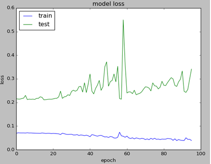
Sometimes validation loss is getting high value and this prevents from seeing other data on the chart. I added few lines of code to cut high values so you can see all details on chart.

import matplotlib.pyplot as plt
import matplotlib.ticker as mtick

T=25
history_val_loss=[]

for x in history.history['val_loss']:
      if x >= T:
             history_val_loss.append (T)
      else:
             history_val_loss.append( x )

plt.figure(6)
plt.plot(history.history['loss'])
plt.plot(history_val_loss)
plt.title('model loss adjusted')
plt.ylabel('loss')
plt.xlabel('epoch')
plt.legend(['train', 'test'], loc='upper left')

Below is the example of charts. Left graph is not showing any details except high value point because of the scale. Note that graphs are obtained from different tests.

2. Early Stopping

Early stopping is allowing to save time on not running tests when a monitored quantity has stopped improving. Here is how it can be coded:

earlystop = EarlyStopping(monitor='val_loss', min_delta=0.0001, patience=80,  verbose=1, mode='min')
callbacks_list = [earlystop]

history=model.fit (x_train, y_train, batch_size =1, nb_epoch =1000, shuffle = False, validation_split=0.15, callbacks=callbacks_list)

Here is what arguments mean per Keras documentation [2].

min_delta: minimum change in the monitored quantity to qualify as an improvement, i.e. an absolute change of less than min_delta, will count as no improvement.
patience: number of epochs with no improvement after which training will be stopped.
verbose: verbosity mode.
mode: one of {auto, min, max}. In min mode, training will stop when the quantity monitored has stopped decreasing; in max mode it will stop when the quantity monitored has stopped increasing; in auto mode, the direction is automatically inferred from the name of the monitored quantity.

3. Weight Regularization

Weight regularizer can be used to regularize neural net weights. Here is the example.

from keras.regularizers import L1L2
model.add (LSTM ( 400,  activation = 'relu', inner_activation = 'hard_sigmoid' , bias_regularizer=L1L2(l1=0.01, l2=0.01),  input_shape =(len(cols), 1), return_sequences = False ))

Below are the charts that are showing impact of weight regularizer on loss value :

Without weight regularization validation loss is going more up during the neural net training.

4. Optimizer

Keras software allows to use different optimizers. I was using adam optimizer which is widely used. Here is how it can be used:

adam=optimizers.Adam(lr=0.01, beta_1=0.91, beta_2=0.999, epsilon=None, decay=0.0, amsgrad=True)
model.compile (loss ="mean_squared_error" , optimizer = "adam") 

I found that beta_1=0.89 performed better then suggested 0.91 or other tested values.

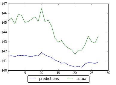
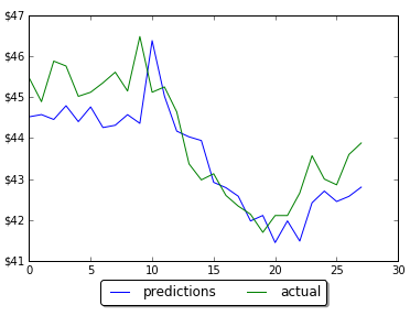
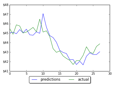
5. Rolling Window Size

Rolling window (in case we use it) also can impact on performance. Too small or too big will drive higher validation loss. Below are charts for different window size (N=4,8,16,18, from left to right). In this case the optimal value was 16 which resulted in 81% accuracy.

I hope you enjoyed this post on different techniques for tuning hyper parameters. If you have any tips or anything else to add, please leave a comment below in the comment box.

Below is the full source code:

import numpy as np
import pandas as pd
from sklearn import preprocessing

import matplotlib.pyplot as plt
import matplotlib.ticker as mtick

from keras.regularizers import L1L2

fname="C:\\Users\\stock data\\GM.csv"
data_csv = pd.read_csv (fname)

#how many data we will use 
# (should not be more than dataset length )
data_to_use= 150

# number of training data
# should be less than data_to_use
train_end =120


total_data=len(data_csv)

#most recent data is in the end 
#so need offset
start=total_data - data_to_use


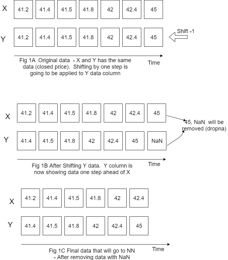
yt = data_csv.iloc [start:total_data ,4]    #Close price
yt_ = yt.shift (-1)   

print (yt_)

data = pd.concat ([yt, yt_], axis =1)
data. columns = ['yt', 'yt_']


N=16    
cols =['yt']
for i in range (N):
  
    data['yt'+str(i)] = list(yt.shift(i+1))
    cols.append ('yt'+str(i))
    
data = data.dropna()
data_original = data
data=data.diff()
data = data.dropna()
    
    
# target variable - closed price
# after shifting
y = data ['yt_']
x = data [cols]

   
scaler_x = preprocessing.MinMaxScaler ( feature_range =( -1, 1))
x = np. array (x).reshape ((len( x) ,len(cols)))
x = scaler_x.fit_transform (x)

scaler_y = preprocessing. MinMaxScaler ( feature_range =( -1, 1))
y = np.array (y).reshape ((len( y), 1))
y = scaler_y.fit_transform (y)

    
x_train = x [0: train_end,]
x_test = x[ train_end +1:len(x),]    
y_train = y [0: train_end] 
y_test = y[ train_end +1:len(y)]  

x_train = x_train.reshape (x_train. shape + (1,)) 
x_test = x_test.reshape (x_test. shape + (1,))

from keras.models import Sequential
from keras.layers.core import Dense
from keras.layers.recurrent import LSTM
from keras.layers import  Dropout
from keras import optimizers

from numpy.random import seed
seed(1)
from tensorflow import set_random_seed
set_random_seed(2)

from keras import regularizers

from keras.callbacks import EarlyStopping


earlystop = EarlyStopping(monitor='val_loss', min_delta=0.0001, patience=80,  verbose=1, mode='min')
callbacks_list = [earlystop]

model = Sequential ()
model.add (LSTM ( 400,  activation = 'relu', inner_activation = 'hard_sigmoid' , bias_regularizer=L1L2(l1=0.01, l2=0.01),  input_shape =(len(cols), 1), return_sequences = False ))
model.add(Dropout(0.3))
model.add (Dense (output_dim =1, activation = 'linear', activity_regularizer=regularizers.l1(0.01)))
adam=optimizers.Adam(lr=0.01, beta_1=0.89, beta_2=0.999, epsilon=None, decay=0.0, amsgrad=True)
model.compile (loss ="mean_squared_error" , optimizer = "adam") 
history=model.fit (x_train, y_train, batch_size =1, nb_epoch =1000, shuffle = False, validation_split=0.15, callbacks=callbacks_list)


y_train_back=scaler_y.inverse_transform (np. array (y_train). reshape ((len( y_train), 1)))
plt.figure(1)
plt.plot (y_train_back)


fmt = '%.1f'
tick = mtick.FormatStrFormatter(fmt)
ax = plt.axes()
ax.yaxis.set_major_formatter(tick)
print (model.summary())

print(history.history.keys())

T=25
history_val_loss=[]

for x in history.history['val_loss']:
      if x >= T:
             history_val_loss.append (T)
      else:
             history_val_loss.append( x )


plt.figure(2)
plt.plot(history.history['loss'])
plt.plot(history.history['val_loss'])
plt.title('model loss')
plt.ylabel('loss')
plt.xlabel('epoch')
plt.legend(['train', 'test'], loc='upper left')
fmt = '%.1f'
tick = mtick.FormatStrFormatter(fmt)
ax = plt.axes()
ax.yaxis.set_major_formatter(tick)



plt.figure(6)
plt.plot(history.history['loss'])
plt.plot(history_val_loss)
plt.title('model loss adjusted')
plt.ylabel('loss')
plt.xlabel('epoch')
plt.legend(['train', 'test'], loc='upper left')


score_train = model.evaluate (x_train, y_train, batch_size =1)
score_test = model.evaluate (x_test, y_test, batch_size =1)
print (" in train MSE = ", round( score_train ,4)) 
print (" in test MSE = ", score_test )

pred1 = model.predict (x_test) 
pred1 = scaler_y.inverse_transform (np. array (pred1). reshape ((len( pred1), 1)))
 
prediction_data = pred1[-1]     
model.summary()
print ("Inputs: {}".format(model.input_shape))
print ("Outputs: {}".format(model.output_shape))
print ("Actual input: {}".format(x_test.shape))
print ("Actual output: {}".format(y_test.shape))

print ("prediction data:")
print (prediction_data)

y_test = scaler_y.inverse_transform (np. array (y_test). reshape ((len( y_test), 1)))
print ("y_test:")
print (y_test)

act_data = np.array([row[0] for row in y_test])

fmt = '%.1f'
tick = mtick.FormatStrFormatter(fmt)
ax = plt.axes()
ax.yaxis.set_major_formatter(tick)

plt.figure(3)
plt.plot( y_test, label="actual")
plt.plot(pred1, label="predictions")

print ("act_data:")
print (act_data)

print ("pred1:")
print (pred1)

plt.legend(loc='upper center', bbox_to_anchor=(0.5, -0.05),
          fancybox=True, shadow=True, ncol=2)


fmt = '$%.1f'
tick = mtick.FormatStrFormatter(fmt)
ax = plt.axes()
ax.yaxis.set_major_formatter(tick)

def moving_test_window_preds(n_future_preds):

    ''' n_future_preds - Represents the number of future predictions we want to make
                         This coincides with the number of windows that we will move forward
                         on the test data
    '''
    preds_moving = []                                    # Store the prediction made on each test window
    moving_test_window = [x_test[0,:].tolist()]          # First test window
    moving_test_window = np.array(moving_test_window)    
   
    for i in range(n_future_preds):
      
      
        preds_one_step = model.predict(moving_test_window) 
        preds_moving.append(preds_one_step[0,0]) 
                       
        preds_one_step = preds_one_step.reshape(1,1,1) 
        moving_test_window = np.concatenate((moving_test_window[:,1:,:], preds_one_step), axis=1) # new moving test window, where the first element from the window has been removed and the prediction  has been appended to the end
        

    print ("pred moving before scaling:")
    print (preds_moving)
                                         
    preds_moving = scaler_y.inverse_transform((np.array(preds_moving)).reshape(-1, 1))
    
    print ("pred moving after scaling:")
    print (preds_moving)
    return preds_moving
    
print ("do moving test predictions for next 22 days:")    
preds_moving = moving_test_window_preds(22)


count_correct=0
error =0
for i in range (len(y_test)):
    error=error + ((y_test[i]-preds_moving[i])**2) / y_test[i]

 
    if y_test[i] >=0 and preds_moving[i] >=0 :
        count_correct=count_correct+1
    if y_test[i] < 0 and preds_moving[i] < 0 :
        count_correct=count_correct+1

accuracy_in_change =  count_correct / (len(y_test) )

plt.figure(4)
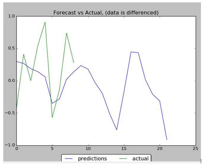
plt.title("Forecast vs Actual, (data is differenced)")          
plt.plot(preds_moving, label="predictions")
plt.plot(y_test, label="actual")
plt.legend(loc='upper center', bbox_to_anchor=(0.5, -0.05),
          fancybox=True, shadow=True, ncol=2)


print ("accuracy_in_change:")
print (accuracy_in_change)

ind=data_original.index.values[0] + data_original.shape[0] -len(y_test)-1
prev_starting_price = data_original.loc[ind,"yt_"]
preds_moving_before_diff =  [0 for x in range(len(preds_moving))]

for i in range (len(preds_moving)):
    if (i==0):
        preds_moving_before_diff[i]=prev_starting_price + preds_moving[i]
    else:
        preds_moving_before_diff[i]=preds_moving_before_diff[i-1]+preds_moving[i]


y_test_before_diff = [0 for x in range(len(y_test))]

for i in range (len(y_test)):
    if (i==0):
        y_test_before_diff[i]=prev_starting_price + y_test[i]
    else:
        y_test_before_diff[i]=y_test_before_diff[i-1]+y_test[i]


plt.figure(5)
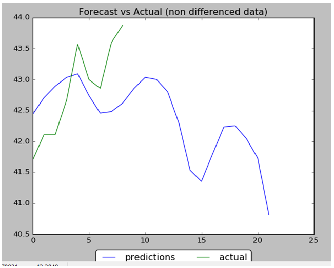
plt.title("Forecast vs Actual (non differenced data)")
plt.plot(preds_moving_before_diff, label="predictions")
plt.plot(y_test_before_diff, label="actual")
plt.legend(loc='upper center', bbox_to_anchor=(0.5, -0.05),
          fancybox=True, shadow=True, ncol=2)
plt.show()

References
1. Enhancing Neural Network Models for Knowledge Base Completion
2. Usage of callbacks
3. Rolling Window Regression: a Simple Approach for Time Series Next value Predictions