Python Scripts Archives - Page 2 of 10 - Machine Learning Applications

Machine Learning Stock Market Prediction with LSTM Keras

April 3, 2018April 5, 2018 by owygs156

In the previous posts [1,2] I created script for machine learning stock market price on next day prediction. But it was pointed by readers that in stock market prediction, it is more important to know the trend: will the stock go up or down. So I updated the script to predict difference between today and yesterday prices. If it is negative the stock price will go down, if positive it will go up. Below will be described implemented modifications.

Data inputting

Data from previous days are entered as features through additional columns. The number of columns can be changed through parameter N in the beginning of script. So for example for day 20 the input will contain data for day 21 as target and data for days 20, 19,18,17… 20-N
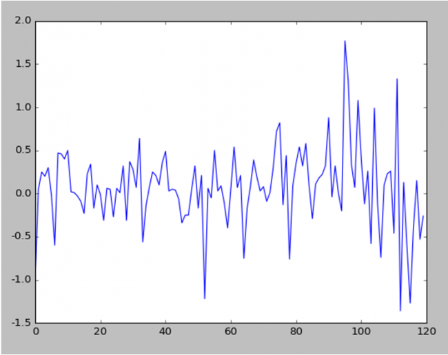
Also added differencing before scaling. Differencing helped to improve performance of network. It also makes easy to get changes from previous day. In the end the differenced data inverted back.

Below is the stock data prices after applying differencing (subtructing previous day stock data price from current day)

Predicting future changes

I used moving_test_window_preds function. Inside of this function the script within loop is adding new prediction to “moving window” array and removing first element from it. This is based on example from blog post on forecasting time series with LSTM[4].
So the script is predicting future day data based on the previous known data in the “moving window”, updating known data and starting again. The performance evaluated by comparing predicted data with test (not used before) data.

LSTM Configuration

The LSTM network is constructed as following:

model = Sequential ()
input_shape =(len(cols), 1) ))
model.add (LSTM ( 400,  activation = 'relu', inner_activation = 'hard_sigmoid' , bias_regularizer=L1L2(l1=0.01, l2=0.01),  input_shape =(len(cols), 1), return_sequences = False ))
model.add(Dropout(0.3))
from keras import optimizers
model.add (Dense (output_dim =1, activation = 'linear', activity_regularizer=regularizers.l1(0.01)))
adam=optimizers.Adam(lr=0.01, beta_1=0.89, beta_2=0.999, epsilon=None, decay=0.0, amsgrad=True)
model.compile (loss ="mean_squared_error" , optimizer = "adam") 
history=model.fit (x_train, y_train, batch_size =1, nb_epoch =1400, shuffle = False, validation_split=0.15)

Weight regularization together with differencing helped to decrease overfitting.

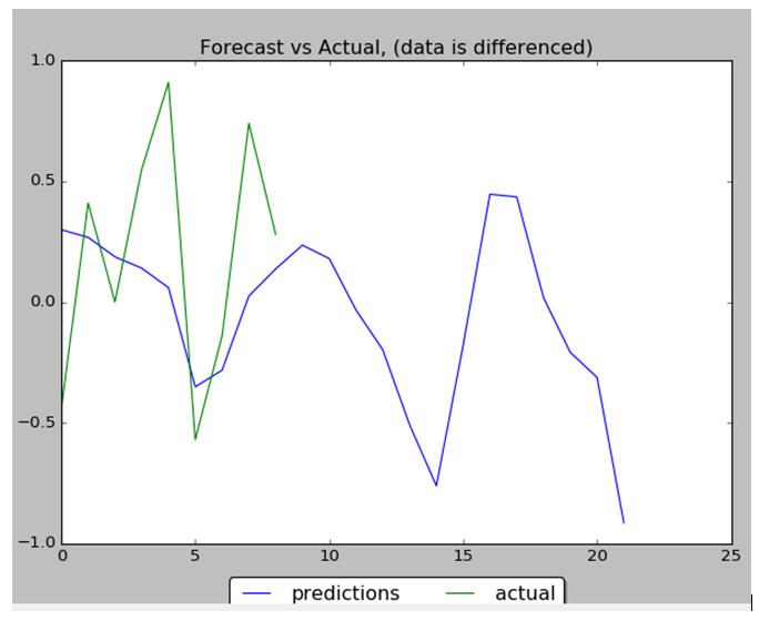
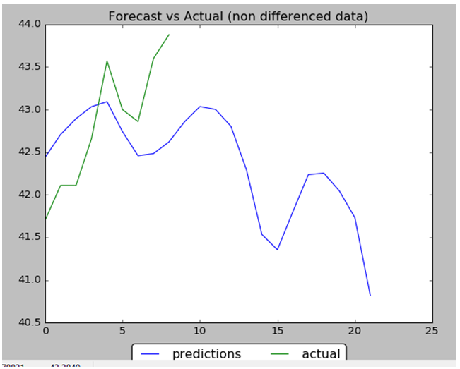
Results

Performance of NN is 88% : 8 correct data out of 9. Below are the data charts that comparing predicted data (9 first days from 22 total days) with actual test data. Below you can find output chart and full python source code.

import numpy as np
import pandas as pd
from sklearn import preprocessing
 
import matplotlib.pyplot as plt
import matplotlib.ticker as mtick
 
from keras.regularizers import L1L2
 
fname="C:\\Users\\Leo\\Desktop\\A\\WS\\stock data analysis 2017\\GM.csv"
data_csv = pd.read_csv (fname)
 
#how many data we will use 
# (should not be more than dataset length )
data_to_use= 150
 
# number of training data
# should be less than data_to_use
train_end =120
 
 
total_data=len(data_csv)
 
#most recent data is in the end 
#so need offset
start=total_data - data_to_use
 
 
yt = data_csv.iloc [start:total_data ,4]    #Close price
yt_ = yt.shift (-1)   
 
print (yt_)
 
data = pd.concat ([yt, yt_], axis =1)
data. columns = ['yt', 'yt_']
 
 
N=18   
cols =['yt']
for i in range (N):
   
    data['yt'+str(i)] = list(yt.shift(i+1))
    cols.append ('yt'+str(i))
     
data = data.dropna()
data_original = data
data=data.diff()
data = data.dropna()
     
     
# target variable - closed price
# after shifting
y = data ['yt_']
x = data [cols]
 
    
scaler_x = preprocessing.MinMaxScaler ( feature_range =( -1, 1))
x = np. array (x).reshape ((len( x) ,len(cols)))
x = scaler_x.fit_transform (x)
 
scaler_y = preprocessing. MinMaxScaler ( feature_range =( -1, 1))
y = np.array (y).reshape ((len( y), 1))
y = scaler_y.fit_transform (y)
 
     
x_train = x [0: train_end,]
x_test = x[ train_end +1:len(x),]    
y_train = y [0: train_end] 
y_test = y[ train_end +1:len(y)]  
 
x_train = x_train.reshape (x_train. shape + (1,)) 
x_test = x_test.reshape (x_test. shape + (1,))
 
from keras.models import Sequential
from keras.layers.core import Dense
from keras.layers.recurrent import LSTM
from keras.layers import  Dropout
from keras import optimizers
 
from numpy.random import seed
seed(1)
from tensorflow import set_random_seed
set_random_seed(2)
 
from keras import regularizers
 
 
model = Sequential ()
model.add (LSTM ( 400,  activation = 'relu', inner_activation = 'hard_sigmoid' , bias_regularizer=L1L2(l1=0.01, l2=0.01),  input_shape =(len(cols), 1), return_sequences = False ))
model.add(Dropout(0.3))
model.add (Dense (output_dim =1, activation = 'linear', activity_regularizer=regularizers.l1(0.01)))
adam=optimizers.Adam(lr=0.01, beta_1=0.89, beta_2=0.999, epsilon=None, decay=0.0, amsgrad=True)
model.compile (loss ="mean_squared_error" , optimizer = "adam") 
history=model.fit (x_train, y_train, batch_size =1, nb_epoch =1400, shuffle = False, validation_split=0.15)
 
 
y_train_back=scaler_y.inverse_transform (np. array (y_train). reshape ((len( y_train), 1)))
plt.figure(1)
plt.plot (y_train_back)
 
 
fmt = '%.1f'
tick = mtick.FormatStrFormatter(fmt)
ax = plt.axes()
ax.yaxis.set_major_formatter(tick)
print (model.summary())
print(history.history.keys())
 
plt.figure(2)
plt.plot(history.history['loss'])
plt.plot(history.history['val_loss'])
plt.title('model loss')
plt.ylabel('loss')
plt.xlabel('epoch')
plt.legend(['train', 'test'], loc='upper left')
fmt = '%.1f'
tick = mtick.FormatStrFormatter(fmt)
ax = plt.axes()
ax.yaxis.set_major_formatter(tick)
 
score_train = model.evaluate (x_train, y_train, batch_size =1)
score_test = model.evaluate (x_test, y_test, batch_size =1)
print (" in train MSE = ", round( score_train ,4)) 
print (" in test MSE = ", score_test )
 
pred1 = model.predict (x_test) 
pred1 = scaler_y.inverse_transform (np. array (pred1). reshape ((len( pred1), 1)))
  
prediction_data = pred1[-1]     
model.summary()
print ("Inputs: {}".format(model.input_shape))
print ("Outputs: {}".format(model.output_shape))
print ("Actual input: {}".format(x_test.shape))
print ("Actual output: {}".format(y_test.shape))
 
print ("prediction data:")
print (prediction_data)
 
y_test = scaler_y.inverse_transform (np. array (y_test). reshape ((len( y_test), 1)))
print ("y_test:")
print (y_test)
 
act_data = np.array([row[0] for row in y_test])
 
fmt = '%.1f'
tick = mtick.FormatStrFormatter(fmt)
ax = plt.axes()
ax.yaxis.set_major_formatter(tick)
 
plt.figure(3)
plt.plot( y_test, label="actual")
plt.plot(pred1, label="predictions")
 
print ("act_data:")
print (act_data)
 
print ("pred1:")
print (pred1)
 
plt.legend(loc='upper center', bbox_to_anchor=(0.5, -0.05),
          fancybox=True, shadow=True, ncol=2)
 
 
fmt = '$%.1f'
tick = mtick.FormatStrFormatter(fmt)
ax = plt.axes()
ax.yaxis.set_major_formatter(tick)
 
def moving_test_window_preds(n_future_preds):
 
    ''' n_future_preds - Represents the number of future predictions we want to make
                         This coincides with the number of windows that we will move forward
                         on the test data
    '''
    preds_moving = []                                    # Store the prediction made on each test window
    moving_test_window = [x_test[0,:].tolist()]          # First test window
    moving_test_window = np.array(moving_test_window)    
    
    for i in range(n_future_preds):
       
       
        preds_one_step = model.predict(moving_test_window) 
        preds_moving.append(preds_one_step[0,0]) 
                        
        preds_one_step = preds_one_step.reshape(1,1,1) 
        moving_test_window = np.concatenate((moving_test_window[:,1:,:], preds_one_step), axis=1) # new moving test window, where the first element from the window has been removed and the prediction  has been appended to the end
         
 
    print ("pred moving before scaling:")
    print (preds_moving)
                                          
    preds_moving = scaler_y.inverse_transform((np.array(preds_moving)).reshape(-1, 1))
     
    print ("pred moving after scaling:")
    print (preds_moving)
    return preds_moving
     
print ("do moving test predictions for next 22 days:")    
preds_moving = moving_test_window_preds(22)
 
 
count_correct=0
error =0
for i in range (len(y_test)):
    error=error + ((y_test[i]-preds_moving[i])**2) / y_test[i]
 
  
    if y_test[i] >=0 and preds_moving[i] >=0 :
        count_correct=count_correct+1
    if y_test[i] < 0 and preds_moving[i] < 0 :
        count_correct=count_correct+1
 
accuracy_in_change =  count_correct / (len(y_test) )
 
plt.figure(4)
plt.title("Forecast vs Actual, (data is differenced)")          
plt.plot(preds_moving, label="predictions")
plt.plot(y_test, label="actual")
plt.legend(loc='upper center', bbox_to_anchor=(0.5, -0.05),
          fancybox=True, shadow=True, ncol=2)
 
 
print ("accuracy_in_change:")
print (accuracy_in_change)
 
ind=data_original.index.values[0] + data_original.shape[0] -len(y_test)-1
prev_starting_price = data_original.loc[ind,"yt_"]
preds_moving_before_diff =  [0 for x in range(len(preds_moving))]
 
for i in range (len(preds_moving)):
    if (i==0):
        preds_moving_before_diff[i]=prev_starting_price + preds_moving[i]
    else:
        preds_moving_before_diff[i]=preds_moving_before_diff[i-1]+preds_moving[i]
 
 
y_test_before_diff = [0 for x in range(len(y_test))]
 
for i in range (len(y_test)):
    if (i==0):
        y_test_before_diff[i]=prev_starting_price + y_test[i]
    else:
        y_test_before_diff[i]=y_test_before_diff[i-1]+y_test[i]
 
 
plt.figure(5)
plt.title("Forecast vs Actual (non differenced data)")
plt.plot(preds_moving_before_diff, label="predictions")
plt.plot(y_test_before_diff, label="actual")
plt.legend(loc='upper center', bbox_to_anchor=(0.5, -0.05),
          fancybox=True, shadow=True, ncol=2)
plt.show()

References
1. Time Series Prediction with LSTM and Keras for Multiple Steps Ahead
2. Machine Learning Stock Prediction with LSTM and Keras
3. Data File
4. Using LSTMs to forecast time-series

Time Series Prediction with LSTM and Keras for Multiple Steps Ahead

February 27, 2018April 17, 2018 by owygs156

In this post I will share experiment with Time Series Prediction with LSTM and Keras. LSTM neural network is used in this experiment for multiple steps ahead for stock prices data. The experiment is based on the paper [1]. The authors of the paper examine independent value prediction approach. With this approach a separate model is built for each prediction step. This approach helps to avoid error accumulation problem that we have when we use multi-stage step prediction.

LSTM Implementation

Following this approach I decided to use Long Short-Term Memory network or LSTM network for daily data stock price prediction. LSTM is a type of recurrent neural network used in deep learning. LSTMs have been used to advance the state-of the-art for many difficult problems. [2]

For this time series prediction I selected the number of steps to predict ahead = 3 and built 3 LSTM models with Keras in python. For each model I used different variable (fit0, fit1, fit2) to avoid any “memory leakage” between models.
The model initialization code is the same for all 3 models except changing parameters (number of neurons in LSTM layer)
The architecture of the system is shown on the fig below.

Multiple step prediction with separate neural networks

Here we have 3 LSTM models that are getting same X input data but different target Y data. The target data is shifted by number of steps. If model is forecasting the data stock price for day 2 then Y is shifted by 2 elements.
This happens in the following line when i=1:

1	`yt_` `=` `yt.shift (-i` `-` `1` `)`

The data were obtained from stock prices from Internet.

The number of unit was obtained by running several variations and chosen based on MSE as following:

if i==0:
    units=20
    batch_size=1
if i==1:
    units=15
    batch_size=1
if i==2:
     units=80
     batch_size=1

If you want run more than 3 steps / models you will need to add parameters to the above code. Additionally you will need add model initialization code shown below.

Each LSTM network was constructed as following:

if i == 0 :
         fit0 = Sequential ()
         fit0.add (LSTM (  units , activation = 'tanh', inner_activation = 'hard_sigmoid' , input_shape =(len(cols), 1) ))
         fit0.add(Dropout(0.2))
         fit0.add (Dense (output_dim =1, activation = 'linear'))
         fit0.compile (loss ="mean_squared_error" , optimizer = "adam")  
   
         fit0.fit (x_train, y_train, batch_size =batch_size, nb_epoch =25, shuffle = False)
         train_mse[i] = fit0.evaluate (x_train, y_train, batch_size =batch_size)
         test_mse[i] = fit0.evaluate (x_test, y_test, batch_size =batch_size)
         pred = fit0.predict (x_test) 
         pred = scaler_y.inverse_transform (np. array (pred). reshape ((len( pred), 1)))
            # below is just fo i == 0
         for j in range (len(pred)) :
                  prediction_data[j] = pred[j] 

For each model the code is saving last forecasted number.
Additionally at step i=0 predicted data is saved for comparison with actual data:

prediction_data = np.asarray(prediction_data)
prediction_data = prediction_data.ravel()
 
# shift back by one step
for j in range (len(prediction_data) - 1 ):
    prediction_data[len(prediction_data) - j - 1  ] =  prediction_data[len(prediction_data) - 1 - j - 1]
 
# combine prediction data from first model and last predicted data from each model
prediction_data = np.append(prediction_data, forecast)

The full python source code for time series prediction with LSTM in python is shown here

Data can be found here

Experiment Results

The LSTM neural network was running with the following performance:

train_mse
[0.01846262458218137, 0.009637593373373323, 0.0018845983509225203]
test_mse
[0.01648362025879952, 0.026161141224167357, 0.01774421124347165]

Below is the graph of actual data vs data testing data, including last 3 stock data prices from each model.

Multiple step prediction actual data vs predictions — Multiple step prediction – actual data vs predictions

Accuracy of prediction 98% calculated for last 3 data stock prices (one from each model).

The experiment confirmed that using models (one model for each step) in multistep-ahead time series prediction has advantages. With this method we can adjust parameters of needed LSTM for each step. For example, number of neurons for i=2 was modified to decrease prediction error for this step. And it did not affect predictions for other steps. This is one of machine learning techniques for stock prediction that is described in [1]

References
1. Multistep-ahead Time Series Prediction
2. LSTM: A Search Space Odyssey
3. Deep Time Series Forecasting with Python: An Intuitive Introduction to Deep Learning for Applied Time Series Modeling

Prediction on Next Stock Market Correction

February 24, 2018March 8, 2018 by owygs156

On Feb. 6, 2018, the stock market officially entered “correction” territory. A stock market correction is defined as a drop of at least 10% or more for an index or stock from its recent high. [1] During one week the stock data prices (closed price) were decreasing for many stocks. Are there any signals that can be used to predict next stock market correction?

I pulled historical data from 20 stocks selected randomly and then created python program that counts how many stocks (closed price) were decreased, increased or did not change for each day (comparing with previous day). The numbers then converted into percentage. So if all 20 stock closed prices decreased at some day it would be 100%. For now I was just looking at % of decreased stocks per day. Below is the graph for decreasing stocks. Highlighted zone A is when we many decreasing stocks during the correction.

Number of decreasing stocks per day in %

Observations

I did not find good strong signal to predict market correction but probably more analysis needed. However before this correction there was some increasing trend for number of stocks that close at lower prices. This is shown below. On this graph the trend line can be viewed as indicator of stock market direction.

Number-of-decreasing-stocks-per-day-before-correction — Number of decreasing stocks per day before correction in %

Python Source Code to download Stock Data

Here is the script that was used to download data:

from pandas_datareader import data as pdr 
import time   
 
# put below actual symbols as many as you need
symbols=['XXX','XXX', 'XXX', ...... 'XXX']
  
 
def get_data (symbol):
     
    data = pdr.get_data_google(symbol,'1970-01-01','2018-02-19')
    path="C:\\Users\\stocks\\"
    data.to_csv( path + symbol+".csv")
  
    return data
 
 
     
for symbol in symbols:
        get_data(symbol)    
        time.sleep(7)

Script for Stock Data Analysis

Here is the program that takes downloaded data and counts the number of decreased/increased/same stocks per day. The results are saved in the file and also plotted. Plots are shown after source code below.

And here is the link to the data output from the below program.

# -*- coding: utf-8 -*-
 
import os
 
path="C:\\Users\\stocks\\"
from datetime import datetime
import pandas as pd
import numpy as np
 
def days_between(d1, d2):
    d1 = datetime.strptime(d1, "%Y-%m-%d")
    d2 = datetime.strptime(d2, "%Y-%m-%d")
    print (d1)
    print (d2)
    return abs((d2 - d1).days)
 
 
i=10000   # index to replace date
j=20      # index for stock symbols
k=5       # other attributes
data = np.zeros((i,j,k))           
symbols=[]           
 
count=0       
 
# get index of previous trade day
# because there is no trades on weekend or holidays
# need to calculate prvious trade day index instead
# of just subracting 1
def get_previous_ind(row_ind, col_count ):
     
    k=1
    print (str(row_ind) + "   " + str(col_count))
    while True:
        if  data[row_ind-k][col_count][0] == 1:
            return row_ind-k
        else:
            k=k+1
     
        if k > 1000 :
            print ("ERROR: PREVIOUS ROW IS NOT FOUND")
            return -1
 
dates=["" for i in range(10000) ]          
# read the entries
listOfEntries = os.scandir(path)
for entry in  listOfEntries: 
         
     if entry.is_file():
            print(entry.name)
            stock_data = pd.read_csv (str(path) + str(entry.name))
            symbols.append (entry.name)
 
                      
            for index, row in stock_data.iterrows():
                 ind=days_between(row['Date'], "2002-01-01") 
                 
                 dates[ind] = row['Date']
                 data[ind][count][0] = 1
                 data[ind][count][1] = row['Close']
                  
                 if (index > 1):
                     print(entry.name)
                     prev_ind=get_previous_ind(ind, count)
                     delta= 1000*(row['Close'] - data[prev_ind][count][1])
                     change=0
                     if (delta > 0) :
                          change = 1
                     if (delta < 0) :
                          change = -1
                     data[ind][count][3] = change  
                     data[ind][count][4] = 1  
                 
                  
            count=count+1                     
 
     
upchange=[0 for i in range(10000)]
downchange=[0 for i in range(10000)]
zerochange=[0 for i in range(10000)]
datesnew = ["" for i in range(10000) ]
icount=0
for i in range(10000):
       total=0
       for j in range (count):
            
           if data[i][j][4] == 1 :
               datesnew[icount]=dates[i]
               total=total+1
               if (data[i][j][3] ==0):
                       zerochange[icount]=zerochange[icount]+1
               if (data[i][j][3] ==1):
                       upchange[icount]=upchange[icount] + 1
               if (data[i][j][3] == - 1):
                       downchange[icount]=downchange[icount] + 1
          
            
       if (total != 0) :
               upchange[icount]=100* upchange[icount] / total
               downchange[icount]=100* downchange[icount] / total
               zerochange[icount]=100* zerochange[icount] / total    
               print (str(upchange[icount]) + "  " +  str(downchange[icount]) + "  " + str(zerochange[icount]))
               icount=icount+1
 
             
 
df=pd.DataFrame({'Date':datesnew, 'upchange':upchange, 'downchange':downchange, 'zerochange':zerochange })
print (df)
df.to_csv("changes.csv", encoding='utf-8', index=False)               
             
 
import matplotlib.pyplot as plt
 
downchange=downchange[icount-200:icount]
upchange=upchange[icount-200:icount]
zerochange=zerochange[icount-200:icount]
 
 
# Two subplots, the axes array is 1-d
f, axarr = plt.subplots(3, sharex=True)
axarr[0].plot(downchange)
axarr[0].set_title('downchange')
axarr[1].plot(upchange)
axarr[1].set_title('upchange')
axarr[2].plot(zerochange)
axarr[2].set_title('zerochange')
plt.show()

Number of stocks increasing decreasing same in %

References
1. 6 Things You Should Know About a Stock Market Correction
2. How to Predict the Eventual Stock Market Correction Before Anyone Else
3. 4 Ways To Predict Market Performance

How to Create Data Visualization for Association Rules in Data Mining

February 10, 2018February 16, 2018 by owygs156

Association rule learning is used in machine learning for discovering interesting relations between variables. Apriori algorithm is a popular algorithm for association rules mining and extracting frequent itemsets with applications in association rule learning. It has been designed to operate on databases containing transactions, such as purchases by customers of a store (market basket analysis). [1] Besides market basket analysis this algorithm can be applied to other problems. For example in web user navigation domain we can search for rules like customer who visited web page A and page B also visited page C.

Python sklearn library does not have Apriori algorithm but recently I come across post [3] where python library MLxtend was used for Market Basket Analysis. MLxtend has modules for different tasks. In this post I will share how to create data visualization for association rules in data mining using MLxtend for getting association rules and NetworkX module for charting the diagram. First we need to get association rules.

Getting Association Rules from Array Data

To get association rules you can run the following code[4]

dataset = [['Milk', 'Onion', 'Nutmeg', 'Kidney Beans', 'Eggs', 'Yogurt'],
           ['Dill', 'Onion', 'Nutmeg', 'Kidney Beans', 'Eggs', 'Yogurt'],
           ['Milk', 'Apple', 'Kidney Beans', 'Eggs'],
           ['Milk', 'Unicorn', 'Corn', 'Kidney Beans', 'Yogurt'],
           ['Corn', 'Onion', 'Onion', 'Kidney Beans', 'Ice cream', 'Eggs']]
            
            
import pandas as pd
from mlxtend.preprocessing import OnehotTransactions
from mlxtend.frequent_patterns import apriori
 
oht = OnehotTransactions()
oht_ary = oht.fit(dataset).transform(dataset)
df = pd.DataFrame(oht_ary, columns=oht.columns_)
print (df)           
 
frequent_itemsets = apriori(df, min_support=0.6, use_colnames=True)
print (frequent_itemsets)
 
association_rules(frequent_itemsets, metric="confidence", min_threshold=0.7)
rules = association_rules(frequent_itemsets, metric="lift", min_threshold=1.2)
print (rules)
 
"""
Below is the output
    support                     itemsets
0       0.8                       [Eggs]
1       1.0               [Kidney Beans]
2       0.6                       [Milk]
3       0.6                      [Onion]
4       0.6                     [Yogurt]
5       0.8         [Eggs, Kidney Beans]
6       0.6                [Eggs, Onion]
7       0.6         [Kidney Beans, Milk]
8       0.6        [Kidney Beans, Onion]
9       0.6       [Kidney Beans, Yogurt]
10      0.6  [Eggs, Kidney Beans, Onion]
 
             antecedants            consequents  support  confidence  lift
0  (Kidney Beans, Onion)                 (Eggs)      0.6        1.00  1.25
1   (Kidney Beans, Eggs)                (Onion)      0.8        0.75  1.25
2                (Onion)   (Kidney Beans, Eggs)      0.6        1.00  1.25
3                 (Eggs)  (Kidney Beans, Onion)      0.8        0.75  1.25
4                (Onion)                 (Eggs)      0.6        1.00  1.25
5                 (Eggs)                (Onion)      0.8        0.75  1.25
 
"""

Confidence and Support in Data Mining

To select interesting rules we can use best-known constraints which are a minimum thresholds on confidence and support.
Support is an indication of how frequently the itemset appears in the dataset.
Confidence is an indication of how often the rule has been found to be true. [5]

support=rules.as_matrix(columns=['support'])
confidence=rules.as_matrix(columns=['confidence'])

Below is the scatter plot for support and confidence:

Association rules - scatter plot — Association rules – scatter plot

And here is the python code to build scatter plot. Since few points here have the same values I added small random values to show all points.

import random
import matplotlib.pyplot as plt
 
 
for i in range (len(support)):
   support[i] = support[i] + 0.0025 * (random.randint(1,10) - 5) 
   confidence[i] = confidence[i] + 0.0025 * (random.randint(1,10) - 5)
 
plt.scatter(support, confidence,   alpha=0.5, marker="*")
plt.xlabel('support')
plt.ylabel('confidence') 
plt.show()

How to Create Data Visualization with NetworkX for Association Rules in Data Mining

To represent association rules as diagram, NetworkX python library is utilized in this post. Here is the association rule example :
(Kidney Beans, Onion) ==> (Eggs)

Directed graph below is built for this rule and shown below. Arrows are drawn as just thicker blue stubs. The node with R0 identifies one rule, and it will have always incoming and outcoming edges. Incoming edge(s) will represent antecedants and the stub (arrow) will be next to node.

Below is the example of graph for all rules extracted from example dataset.

Here is the source code to build association rules with NetworkX. To call function use draw_graph(rules, 6)

def draw_graph(rules, rules_to_show):
  import networkx as nx  
  G1 = nx.DiGraph()
   
  color_map=[]
  N = 50
  colors = np.random.rand(N)    
  strs=['R0', 'R1', 'R2', 'R3', 'R4', 'R5', 'R6', 'R7', 'R8', 'R9', 'R10', 'R11']   
   
   
  for i in range (rules_to_show):      
    G1.add_nodes_from(["R"+str(i)])
    
     
    for a in rules.iloc[i]['antecedants']:
                
        G1.add_nodes_from([a])
        
        G1.add_edge(a, "R"+str(i), color=colors[i] , weight = 2)
       
    for c in rules.iloc[i]['consequents']:
             
            G1.add_nodes_from()
            
            G1.add_edge("R"+str(i), c, color=colors[i],  weight=2)
 
  for node in G1:
       found_a_string = False
       for item in strs: 
           if node==item:
                found_a_string = True
       if found_a_string:
            color_map.append('yellow')
       else:
            color_map.append('green')       
 
 
   
  edges = G1.edges()
  colors = [G1[u][v]['color'] for u,v in edges]
  weights = [G1[u][v]['weight'] for u,v in edges]
 
  pos = nx.spring_layout(G1, k=16, scale=1)
  nx.draw(G1, pos, edges=edges, node_color = color_map, edge_color=colors, width=weights, font_size=16, with_labels=False)            
   
  for p in pos:  # raise text positions
           pos[p][1] += 0.07
  nx.draw_networkx_labels(G1, pos)
  plt.show()

Data Visualization for Online Retail Data Set

To get real feeling and testing on visualization we can take available online retail store dataset[6] and apply the code for association rules graph. For downloading retail data and formatting some columns the code from [3] was used.

Below are the result of scatter plot for support and confidence. To build the scatter plot seaborn library was used this time. Also you can find below visualization for association rules (first 10 rules) for retail data set.

Here is the python full source code for data visualization association rules in data mining.

100

101

102

103

104

105

106

107

108

109

110

111

112

113

114

115

116

117

118

119

120

121

122

123

124

125

126

127

128

129

130

131

132

133

134

135

136

137

138

139

140

141

142

143

144

145

dataset = [['Milk', 'Onion', 'Nutmeg', 'Kidney Beans', 'Eggs', 'Yogurt'],
           ['Dill', 'Onion', 'Nutmeg', 'Kidney Beans', 'Eggs', 'Yogurt'],
           ['Milk', 'Apple', 'Kidney Beans', 'Eggs'],
           ['Milk', 'Unicorn', 'Corn', 'Kidney Beans', 'Yogurt'],
           ['Corn', 'Onion', 'Onion', 'Kidney Beans', 'Ice cream', 'Eggs']]
            
            
import pandas as pd
from mlxtend.preprocessing import OnehotTransactions
from mlxtend.frequent_patterns import apriori
 
oht = OnehotTransactions()
oht_ary = oht.fit(dataset).transform(dataset)
df = pd.DataFrame(oht_ary, columns=oht.columns_)
print (df)           
 
frequent_itemsets = apriori(df, min_support=0.6, use_colnames=True)
print (frequent_itemsets)
 
from mlxtend.frequent_patterns import association_rules
 
association_rules(frequent_itemsets, metric="confidence", min_threshold=0.7)
rules = association_rules(frequent_itemsets, metric="lift", min_threshold=1.2)
print (rules)
 
support=rules.as_matrix(columns=['support'])
confidence=rules.as_matrix(columns=['confidence'])
 
 
import random
import matplotlib.pyplot as plt
 
 
for i in range (len(support)):
   support[i] = support[i] + 0.0025 * (random.randint(1,10) - 5) 
   confidence[i] = confidence[i] + 0.0025 * (random.randint(1,10) - 5)
 
plt.scatter(support, confidence,   alpha=0.5, marker="*")
plt.xlabel('support')
plt.ylabel('confidence') 
plt.show()
 
import numpy as np
 
def draw_graph(rules, rules_to_show):
  import networkx as nx  
  G1 = nx.DiGraph()
   
  color_map=[]
  N = 50
  colors = np.random.rand(N)    
  strs=['R0', 'R1', 'R2', 'R3', 'R4', 'R5', 'R6', 'R7', 'R8', 'R9', 'R10', 'R11']   
   
   
  for i in range (rules_to_show):      
    G1.add_nodes_from(["R"+str(i)])
    
     
    for a in rules.iloc[i]['antecedants']:
                
        G1.add_nodes_from([a])
        
        G1.add_edge(a, "R"+str(i), color=colors[i] , weight = 2)
       
    for c in rules.iloc[i]['consequents']:
             
            G1.add_nodes_from()
            
            G1.add_edge("R"+str(i), c, color=colors[i],  weight=2)
 
  for node in G1:
       found_a_string = False
       for item in strs: 
           if node==item:
                found_a_string = True
       if found_a_string:
            color_map.append('yellow')
       else:
            color_map.append('green')       
 
 
   
  edges = G1.edges()
  colors = [G1[u][v]['color'] for u,v in edges]
  weights = [G1[u][v]['weight'] for u,v in edges]
 
  pos = nx.spring_layout(G1, k=16, scale=1)
  nx.draw(G1, pos, edges=edges, node_color = color_map, edge_color=colors, width=weights, font_size=16, with_labels=False)            
   
  for p in pos:  # raise text positions
           pos[p][1] += 0.07
  nx.draw_networkx_labels(G1, pos)
  plt.show()
 
     
draw_graph (rules, 6)   
 
 
df = pd.read_excel('http://archive.ics.uci.edu/ml/machine-learning-databases/00352/Online%20Retail.xlsx')
 
 
df['Description'] = df['Description'].str.strip()
df.dropna(axis=0, subset=['InvoiceNo'], inplace=True)
df['InvoiceNo'] = df['InvoiceNo'].astype('str')
df = df[~df['InvoiceNo'].str.contains('C')]
 
basket = (df[df['Country'] =="France"]
          .groupby(['InvoiceNo', 'Description'])['Quantity']
          .sum().unstack().reset_index().fillna(0)
          .set_index('InvoiceNo'))
 
def encode_units(x):
    if x <= 0:
        return 0
    if x >= 1:
        return 1
 
basket_sets = basket.applymap(encode_units)
basket_sets.drop('POSTAGE', inplace=True, axis=1)
 
frequent_itemsets = apriori(basket_sets, min_support=0.07, use_colnames=True)
 
rules = association_rules(frequent_itemsets, metric="lift", min_threshold=1)
rules.head()
 
print (rules)
 
 
 
support=rules.as_matrix(columns=['support'])
confidence=rules.as_matrix(columns=['confidence'])
 
import seaborn as sns1
 
for i in range (len(support)):
    support[i] = support[i] 
    confidence[i] = confidence[i] 
     
plt.title('Association Rules')
plt.xlabel('support')
plt.ylabel('confidence')    
sns1.regplot(x=support, y=confidence, fit_reg=False)
 
plt.gcf().clear()
draw_graph (rules, 10)  

References

1. MLxtend Apriori
2. mlxtend-latest
3. Introduction to Market Basket Analysis in Python
4. MLxtends-documentation
5. Association rule learning
6. Online Retail Data Set

Machine Learning Stock Prediction with LSTM and Keras – Python Source Code

January 20, 2018March 2, 2018 by owygs156

Python Source Code for Machine Learning Stock Prediction with LSTM and Keras – Python Source Code with LSTM and Keras Below is the code for machine learning stock prediction with LSTM neural network.

# -*- coding: utf-8 -*-
 
import numpy as np
import pandas as pd
from sklearn import preprocessing
import matplotlib.pyplot as plt
 
 
fname="C:\\Users\\stock_data.csv"
data_csv = pd.read_csv (fname)
 
#how many data we will use 
# (should not be more than dataset length )
data_to_use= 100
 
# number of training data
# should be less than data_to_use
train_end =70
 
 
total_data=len(data_csv)
 
#most recent data is in the end 
#so need offset
start=total_data - data_to_use
 
 
#currently doing prediction only for 1 step ahead
steps_to_predict =1
 
  
yt = data_csv.iloc [start:total_data ,4]    #Close price
yt1 = data_csv.iloc [start:total_data ,1]   #Open
yt2 = data_csv.iloc [start:total_data ,2]   #High
yt3 = data_csv.iloc [start:total_data ,3]   #Low
vt = data_csv.iloc [start:total_data ,6]    # volume
 
 
print ("yt head :")
print (yt.head())
 
yt_ = yt.shift (-1)
     
data = pd.concat ([yt, yt_, vt, yt1, yt2, yt3], axis =1)
data. columns = ['yt', 'yt_', 'vt', 'yt1', 'yt2', 'yt3']
     
data = data.dropna()
     
print (data)
     
# target variable - closed price
# after shifting
y = data ['yt_']
 
        
#       closed,  volume,   open,  high,   low    
cols =['yt',    'vt',  'yt1', 'yt2', 'yt3']
x = data [cols]
 
   
    
scaler_x = preprocessing.MinMaxScaler ( feature_range =( -1, 1))
x = np. array (x).reshape ((len( x) ,len(cols)))
x = scaler_x.fit_transform (x)
 
    
scaler_y = preprocessing. MinMaxScaler ( feature_range =( -1, 1))
y = np.array (y).reshape ((len( y), 1))
y = scaler_y.fit_transform (y)
 
     
x_train = x [0: train_end,]
x_test = x[ train_end +1:len(x),]    
y_train = y [0: train_end] 
y_test = y[ train_end +1:len(y)]  
x_train = x_train.reshape (x_train. shape + (1,)) 
x_test = x_test.reshape (x_test. shape + (1,))
 
     
     
 
from keras.models import Sequential
from keras.layers.core import Dense
from keras.layers.recurrent import LSTM
from keras.layers import  Dropout
 
 
seed =2016
np.random.seed (seed)
fit1 = Sequential ()
fit1.add (LSTM (  1000 , activation = 'tanh', inner_activation = 'hard_sigmoid' , input_shape =(len(cols), 1) ))
fit1.add(Dropout(0.2))
fit1.add (Dense (output_dim =1, activation = 'linear'))
 
fit1.compile (loss ="mean_squared_error" , optimizer = "adam")   
fit1.fit (x_train, y_train, batch_size =16, nb_epoch =25, shuffle = False)
 
print (fit1.summary())
 
score_train = fit1.evaluate (x_train, y_train, batch_size =1)
score_test = fit1.evaluate (x_test, y_test, batch_size =1)
print (" in train MSE = ", round( score_train ,4)) 
print (" in test MSE = ", score_test )
 
    
pred1 = fit1.predict (x_test) 
pred1 = scaler_y.inverse_transform (np. array (pred1). reshape ((len( pred1), 1)))
     
  
 
  
prediction_data = pred1[-1]     
    
 
fit1.summary()
print ("Inputs: {}".format(fit1.input_shape))
print ("Outputs: {}".format(fit1.output_shape))
print ("Actual input: {}".format(x_test.shape))
print ("Actual output: {}".format(y_test.shape))
   
 
print ("prediction data:")
print (prediction_data)
 
 
print ("actual data")
x_test = scaler_x.inverse_transform (np. array (x_test). reshape ((len( x_test), len(cols))))
print (x_test)
 
 
plt.plot(pred1, label="predictions")
 
 
y_test = scaler_y.inverse_transform (np. array (y_test). reshape ((len( y_test), 1)))
plt.plot( [row[0] for row in y_test], label="actual")
 
plt.legend(loc='upper center', bbox_to_anchor=(0.5, -0.05),
          fancybox=True, shadow=True, ncol=2)
 
import matplotlib.ticker as mtick
fmt = '$%.0f'
tick = mtick.FormatStrFormatter(fmt)
 
ax = plt.axes()
ax.yaxis.set_major_formatter(tick)
 
 
plt.show()

References
1. Machine Learning Stock Prediction with LSTM and Keras – Python Source Code with LSTM and Keras

Data inputting

Predicting future changes

LSTM Configuration

Results

Share this:

LSTM Implementation

Experiment Results

Share this:

Observations

Python Source Code to download Stock Data

Script for Stock Data Analysis

Share this:

Getting Association Rules from Array Data

Confidence and Support in Data Mining

How to Create Data Visualization with NetworkX for Association Rules in Data Mining

Data Visualization for Online Retail Data Set

Share this:

Share this: