wavelet transform

If we see in the real world, we will always face the signals which are not changing their stats. Means the change in the data signals are quite slow. But if we compare the 1D- data to the 2D Image data then we can see the 2D images have more drastic change in the magnitude of the pixels due to edges, change in the contrast and the two different things in the same image.

Fourier Transform isn’t Able to Represent the Abrupt Changes Efficiently

So 1D data have slow oscillation but the images have more abrupt changes. These abrupt changing parts are always the interesting for that data as well as the images. They always show more relevant information for the images and the data.

Now, we have great tool for the analysis of the signals and that is the Fourier transform. But, it doesn’t able to represent the abrupt changes efficiently. That’s the demerit of the Fourier transform. The reason for this is that the Fourier transform is made up from the summation of the weighted sin and cosine signals. So, for abrupt changes that transform is less efficient.

Wavelets and Wavelet Transform is Great Tool for Abrupt Data Analysis

For that problem we must find out different bases except the sin and cosine because these bases are not efficient for the abrupt representation. For the solution of these problems, another great tool came and those are the Wavelets and Wavelet transform. A wavelet is the rapidly decaying, wave like oscillation and that is also for the finite duration not like the sin and cosine (They oscillates forever.)

There are number of wavelets and based on the application and on the nature of the data, we can select the wavelet for that application and the data. Here, I have shown some of the well-known types of wavelets.

Figure 1. Well known types of wavelets (Image is from MathWorks)

Now we are going to plot the Morlet in the MATLAB and that is quite easy if you know the basics of the MATLAB.

The equation for the Morlet wavelet is,

Let us plot the Morlet function using MATLAB.

%% Morlet Wavelet functions
lb = -4;% lower bound
ub = 4;% uper bound
n = 1000; % number of points
x = linspace(lb,ub,n);
y = exp(((-1)*(x.^2))./2).*cos(5*x);
figure,plot(x,y,'LineWidth',2)
% title(['Morlet Wavelet']);
title('Morlet Wavelet $$\psi(t) = e^{\frac{-x^2}{2}} \cos(5x)$$','interpreter','latex')

If we plot this wave then we will get the result like below,

Figure 2. Plot of the Morlet in the MATLAB.

We can see that this Morlet can able to represent the drastic changes and we can scale it for more drastic changes like Figure 3(b).

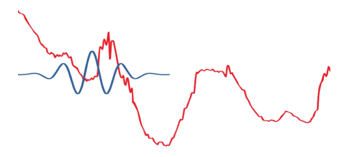
Figure 3a: Less abrupt change and the signal is applied as it is.

Figure 3b: More abrupt change than the figure 3a. and in this case the signal is applied after some scaling.

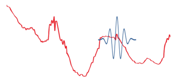
Figure 3c: More abrupt change than the figure 3b. and in this case the signal is applied after very high scaling to represent the very sharp abrupt change.

Now, we have understood what exactly the Wavelets are. These wavelets are the bases for the Wavelet Transform similar like Sine and Cosines are the bases for the Fourier Transform.

The Wavelet Transform

The wavelet transform is the mathematical tool that can able to decomposes a signal into a representation of the signal’s fine details and the trends as the function of time. We can use this transform or this representation to characterize the abrupt changes or transient events, to denoise, to perform many more operations on that.

The main benefit of wavelet transform or methods over traditional Fourier transform or methods are the uses of localized basis functions called as the wavelets and it give more faster computation. Wavelets as being localized basis functions are best for analyzing real physical situations in which a signal have discontinuities, abrupt changes and sharp spikes.

Two major transforms that are very useful to wavelet analysis are the
Continuous Wavelet Transform
Discrete Wavelet Transform

If we see this equation then we will get feel like, oh!! That is very similar to the Fourier transform. Yes, that is very similar to that but here major difference is that ψ(t) and that is the wavelet not the sin and the cosine. Here as a ψ(t), we can take any wavelet that suit best for our applications. Now we will be going to discuss about the uses of the wavelet transform.

The following are applications of wavelet transforms:
Data and image compression
Transient detection
Pattern recognition
Texture analysis
Noise/trend reduction

Wavelet Denoising

In this article we will go through the one application of the wavelet transform and that is denoising of 1-D data.
1-D Data:
I have taken the electrical data through the MATLAB.
load leleccum;
I have taken only the some part of that signal for the process.
s = leleccum(1:3920);

Figure 4. Electrical Signal Lelecum from the MATLAB.

This signal have so much sharp and abrupt changes and we can see some additional noise as well from 2500 to 3500. Here we can use the wavelet transform to denoise this signal.

First, we will perform only the one step Wavelet Decomposition of a Signal. For one step we will get only the two components and one will be approximation and the second will be the detail of the signal. Here I have used the Daubechies wavelet for the wavelet transform.
[cA1,cD1] = dwt(s,’db1′);

This generates the coefficients of the level 1 approximation (cA1) and detail (cD1). This both are coefficients now we can construct the level 1 approximation and the detail as well.

A1 = upcoef('a',cA1,'db1',1,ls);
D1 = upcoef('d',cD1,'db1',1,ls);

If we display it then it will look something like Figure 5. We can see the approximation which are more and less similar to the signal and the details shows the sharp fluctuations of the signal.

Now, we will perform the decomposition of the signal in 3 levels. This decomposition will be the similar to the Figure 6. We can decompose the signal in these levels for more levels of details. Here we will get three level details cD1, cD2 and cD3 and one approximation cA3.

We can create this 3 level decomposition using the “wavedec” function from the MATLAB. This function used for the decomposition of the signal in to multi-level wavelet decomposition.
[C,L] = wavedec(s,3,’db1′);

Here also I have used the Daubechies wavelet. The coefficients of all the components of a third-level decomposition (that is, the third-level approximation and the first three levels of detail) are returned concatenated into one vector, C. Vector L gives the lengths of each component.

Figure 5. Approximation A1 and detail D1 at the first step.

Figure 6. Approximation and the details of the signal till level 3 (Image is from the MATHWORK).
We can extract the level 3 approximation coefficients from C using the “appcoef” function from the MATLAB.

cA3 = appcoef(C,L,'db1',3);

We can extract the level 3 details coefficients from C and L using the “detcoef” function from the MATLAB.

cD3 = detcoef(C,L,3);
cD2 = detcoef(C,L,2);
cD1 = detcoef(C,L,1);

This way we have total three values cA3, cD1, cD2, and cD3. We can reconstruct the approximate and details signals from these coefficients using “wrcoef”.

% To reconstruct the level 3 approximation from C,
A3 = wrcoef('a',C,L,'db1',3);
 
% To reconstruct the details at levels 1, 2 and 3,
D1 = wrcoef('d',C,L,'db1',1);
D2 = wrcoef('d',C,L,'db1',2);
D3 = wrcoef('d',C,L,'db1',3);

If we display this images then it will look something like Figure 7.

Figure 7. Approximation and details at the different levels.

We can use the wavelets to remove noise from a signal but it will requires identifying which component or components have the noise and then recovering the signal without those components. In this example, we have observed that as we increase the number of the steps, the successive approximations become much less and less noisy because more and more high-frequency information is filtered out of the signal.

If we compare the level 3 approximation with the original signal then we can find that level 3 approximation is much more smother than the original signal.

Of course, after removing all the high-frequency information, we will have lost many abrupt information from the original signal. So for optimal de-noising will required a more subtle method and that is called as thresholding. Thresholding involves removing the portion from the details which have higher activity than the certain limits.

What if we limited the strength of the details by restricting their maximum values? This would have the effect of cutting back the noise while leaving the details unaffected through most of their durations. But there’s a better way. We could directly manipulate each vector, setting each element to some fraction of the vectors’ peak or average value. Then we could reconstruct new detail signals D1, D2, and D3 from the thresholded coefficients.

To denoise the image,

[thr,sorh,keepapp] = ddencmp('den','wv',s);
clean = wdencmp('gbl',C,L,'db1',3,thr,sorh,keepapp);

“ddencmp” function gives the default values of the threshold, SORH and KEEPAPP which allows you to keep approximation coefficients. Clean is the denoised signal.

Figure 8. Shows both the original as well as the clean signal.

Figure 8. Original signal with the De-noised signal.

Conclusion:

Wavelet are the great tools for the analysis of the signals and those signals have ability to representation the signal in the great detail. Here we have experimented with the denoising of the electrical signal, we have seen that using only low pass filter may affect the abrupt information of signals. But using the proper process of the wavelet transform we can have great denoised signal.

Wavelets can do much more than the denoising. Popular “.JPEG” encoding format for the images uses the discrete cosine transform for the compression of the images. There is other algorithm JPEG2000 which have great accuracy of the image with great compression. And JPEG2000 algorithm uses the wavelet transform.

Thus wavelets are very useful, so have great time with number of wavelets and may this article helps you to for the understanding of the wavelets.
For whole code in MATLAB and for more exciting projects please visit github.com/MachineLearning-Nerd/Wavelet-Analysis GITHUB repository.