3 Most Useful Examples to Add Interactivity to Graph Data Using Bokeh Library

Bokeh is a Python library for building advanced and modern data visualization web applications. Bokeh allows to add interactive controls like slider, buttons, dropdown menu and so on to the data graphs. Bokeh provides a variety of ways to embed plots and data into HTML documents including generating standalone HTML documents. [6]

There is a sharp increase of popularity for Bokeh data visualization libraries (Fig 1), reflecting the increased interest in machine learning and data science over the last few years.
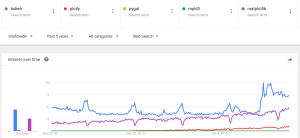
Fig 1. Trend for Bokeh and Other Data Visualizations Libraries. Source: Google Trends

In this post we put together 4 most common examples of data plots using Bokeh. The examples include such popular controls like slider, button. They use loading data from data files which is common situation in practice. The examples show how to add create plot and how to add interactivity using Bokeh and will help to make quick start in using Bokeh.

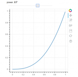
Our first example demonstrates how to add interactivity with slide control. This example is taken from Bokeh documentation [4]. When we change the slider value the line is changing its properties. See Fig 2 for example how the plot is changing. The example is using callbak function attached to slider control.


# -*- coding: utf-8 -*-

from bokeh.layouts import column
from bokeh.models import CustomJS, ColumnDataSource, Slider
from bokeh.plotting import Figure, output_file, show

# fetch and clear the document
from bokeh.io import curdoc
curdoc().clear()

output_file("callback.html")

x = [x*0.005 for x in range(0, 200)]
y = x

source = ColumnDataSource(data=dict(x=x, y=y))

plot = Figure(plot_width=400, plot_height=400)
plot.line('x', 'y', source=source, line_width=3, line_alpha=0.6)

def callback(source=source, window=None):
    data = source.data
    f = cb_obj.value
    x, y = data['x'], data['y']
    for i in range(len(x)):
        y[i] = window.Math.pow(x[i], f)
    source.trigger('change')

slider = Slider(start=0.1, end=4, value=1, step=.1, title="power",
                callback=CustomJS.from_py_func(callback))

layout = column(slider, plot)

show(layout)

Alternatively we can attach callback through the js_on_change method of Bokeh slider model:


callback = CustomJS(args=dict(source=source), code="""
    var data = source.data;
    var f = cb_obj.value
    x = data['x']
    y = data['y']
    for (i = 0; i < x.length; i++) {
        y[i] = Math.pow(x[i], f)
    }
    source.trigger('change');
""")

slider = Slider(start=0.1, end=4, value=1, step=.1, title="power")
slider.js_on_change('value', callback)
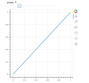
Fig 2A. Initial Data plot
Fig 2B. Data plot after changed slider position

Our second example shows how to use button control. In this example we use Button on_click method to change graph.


# -*- coding: utf-8 -*-

from bokeh.layouts import column
from bokeh.models import CustomJS, ColumnDataSource
from bokeh.plotting import Figure, output_file, show

from bokeh.io import curdoc
curdoc().clear()

from bokeh.models.widgets import Button
output_file("button.html")


x = [x*0.05 for x in range(0, 200)]
y = x

source = ColumnDataSource(data=dict(x=x, y=y))

plot = Figure(plot_width=400, plot_height=400)
plot.line('x', 'y', source=source, line_width=3, line_alpha=0.6)

callback = CustomJS(args=dict(source=source), code="""
    var data = source.data;
    x = data['x']
    y = data['y']
    for (i = 0; i < x.length; i++) {
        y[i] = Math.pow(x[i], 4)
    }
    source.trigger('change');
""")


toggle1 = Button(label="Change Graph", callback=callback, name="1")
layout = column(toggle1 , plot)

show(layout)

Our 3rd example demonstrates how to load data from csv data file. This example is borrowed from stackoverflow [5] In this example we also use button, but here we load data from file to dataframe. We use two buttons, two files and 2 dataframes, the buttons allow to switch between data files and reload the graph.


# -*- coding: utf-8 -*-
from bokeh.io import vplot
import pandas as pd
from bokeh.models import CustomJS, ColumnDataSource
from bokeh.models.widgets import Button
from bokeh.plotting import figure, output_file, show

output_file("load_data_buttons.html")

df1 = pd.read_csv("data_file_1.csv")
df2 = pd.read_csv("data_file_2.csv")

df1.columns = df1.columns.str.strip()
df2.columns = df2.columns.str.strip()
plot = figure(plot_width=400, plot_height=400, title="xxx")
source = ColumnDataSource(data=dict(x=[0, 1], y=[0, 1]))
source2 = ColumnDataSource(data=dict(x1=df1.x.values, y1=df1.y.values, 
                                    x2=df2.x.values, y2=df2.y.values))

plot.line('x', 'y', source=source, line_width=3, line_alpha=0.6)

callback = CustomJS(args=dict(source=source, source2=source2), code="""
        var data = source.get('data');
        var data2 = source2.get('data');
        data['x'] = data2['x' + cb_obj.get("name")];
        data['y'] = data2['y' + cb_obj.get("name")];
        source.trigger('change');
    """)

toggle1 = Button(label="Load data file 1", callback=callback, name="1")
toggle2 = Button(label="Load data file 2", callback=callback, name="2")

layout = vplot(toggle1, toggle2, plot)

show(layout)

As mentioned on the web, Interactive data visualizations turn plots into powerful interfaces for data exploration. [7] The shown above examples demonstrate how to make the graph data interactive and hope will help to make quick start in this direction.

References
1. 5 Python Libraries for Creating Interactive Plots
2. 10 Useful Python Data Visualization Libraries for Any Discipline
3. The Most Popular Language For Machine Learning and Data Science
4. Welcome to Bokeh
5. Load graph data from files on button click with bokeh
6. Embedding Plots and Apps
7. How effective data visualizations let users have a conversation with data


How to Write to a Google Sheet with a Python Script

My post How to Write to a Google Spreadsheet with a Perl Script that was published some time ago is still getting a lot of visitors. This is not surprising as cloud computing is a fast-growing business. Below is the chart of number of searches for phrase “Google Sheet” from Google Trends site. The usage of Google Sheet looks increasing over the years.

“Google Sheet” trend, source Google Trends

So now I decided to look how to use python for Google Sheet.

My interest to this topic also come from the idea to have Adsense and Google Analytics data on the Google Drive and do analysis in python. Keeping files on Google Drive provides access to data from different computers or devices and allows sharing with other people.

Setup
I found good post [2] that helped me quickly setup everything that is needed on Google Drive.

Despite of good instructions I run into the following minor issues:
The file on Google Drive should be shared with the email in secret key file. But this email was not the same email that I use for usual login to Google site. Google created some new email, that is starting with project name. Only when I shared the Google Sheet with that new email it started to work.

The sheet name in the below statement for opening file, for some reason did not take upper case. The actual sheet name was “Sheet1″ but the statement below worked with “sheet1″ only ( s in low case):
sheet = client.open(“filename”).sheet1

Reading and Updating Google Sheet
Here is the small example of python code showing how to read or update Google Sheet.


sheet.update_cell(1, 2, "text 34")

for i in range (2):
    sheet.update_cell(1, i+3, i)

# Returns a list of Cell objects from a specified range.
ar=sheet.range('A1:D1') 
for obj in ar:
    print (obj.value)

Once you get understanding how to do basic operation you can write more complicated code as you need. There are many benefits in using files in the cloud.

Full python source code


# -*- coding: utf-8 -*-
import gspread
from oauth2client.service_account import ServiceAccountCredentials


scope = ['https://spreadsheets.google.com/feeds']
creds = ServiceAccountCredentials.from_json_keyfile_name('client_secret.json', scope)
client = gspread.authorize(creds)

sheet = client.open("File name").sheet1
sheet.update_cell(1, 2, "text 34")

for i in range (2):
    sheet.update_cell(1, i+3, i)

### Returns a list of Cell objects from a specified range.
ar=sheet.range('A1:D1') 
for obj in ar:nprint (obj.value)

Accessing through Web
We can use the same code to access Google Sheet through web. Here is the test example with flask. Python script is navigating through 4 cells, counting the sum and displaying it on the web. To access Google Sheet we used the same code as before.
Below you can find screenshot of web page and Google Sheet.
To run this example you need:
install flask
put this python file and client_secret.json file into the same flask folder
run this python script from command line
run web browser as on the screenshot.

Retrieving the content of Google Sheet through web page with python and flask

Below is the python computer code.


from flask import Flask
app = Flask(__name__)

@app.route('/')
def index():
  return 'Hello World!'


@app.route('/user/')
def user(name):

   import gspread
   from oauth2client.service_account import ServiceAccountCredentials
   scope = ['https://spreadsheets.google.com/feeds']
   creds = ServiceAccountCredentials.from_json_keyfile_name('client_secret.json', scope)
   client = gspread.authorize(creds)

   sheet = client.open("INSERT_REPORT_NAME_HERE").sheet1
   ar=sheet.range('A1:D1')
   sum=0 
   for obj in ar:
       sum = sum + int(obj.value)
   HTML_string='Hello, {}! Total = {}'
   return HTML_string.format(name , str(sum))  

if __name__ == '__main__':
   app.run(debug=True)

References
1. How to Write to a Google Spreadsheet with a Perl Script
2. Google Spreadsheets and Python


Converting Categorical Text Variable into Binary Variables

Sometimes we might need convert categorical feature into multiple binary features. Such situation emerged while I was implementing decision tree with independent categorical variable using python sklearn.tree for the post Building Decision Trees in Python – Handling Categorical Data and it turned out that a text independent variable is not supported.

One of solution would be binary encoding, also called one-hot-encoding when we might code [‘red’,’green’,’blue’] with 3 columns, one for each category, having 1 when the category match and 0 otherwise. [1]

Here we implement the python code that makes such binary encoding. The script looks at text data column and add numerical columns with values 0 or 1 to the original data. If category word exists in the column then it will be 1 in the column for this category, otherwise 0.

The list of categories is initialized in the beginning of the script. Additionally we initialize data source file, number of column with text data, and number of first empty column on right side. The script will add columns on right side starting from first empty column.

The next step in the script is to navigate through each row and do binary conversion and update data.

Below is some example of added binary columns to data input .

Below is full source code.


# -*- coding: utf-8 -*-

import pandas as pd

words = ["adwords", "adsense","mortgage","money","loan"]
data = pd.read_csv('adwords_data5.csv', sep= ',' , header = 0)


total_rows = len(data.index)


y_text_column_index=7
y_column_index=16


for index, w in enumerate(words):
  data[w] = 0   
  col_index=data.columns.get_loc(w)
  
  for x in range (total_rows):
      if w in data.iloc[x,y_text_column_index] :
           data.iloc[x,y_column_index+index]=1
      else :
           data.iloc[x,y_column_index+index]=0  


print (data)

References
1. strings as features in decision tree/random forest
2. Building Decision Trees in Python
3. Building Decision Trees in Python – Handling Categorical Data


Building Decision Trees in Python – Handling Categorical Data

In the post Building Decision Trees in Python we looked at the decision tree with numerical continuous dependent variable. This type of decision trees can be called also regression tree.

But what if we need to use categorical dependent variable? It is still possible to create decision tree and in this post we will look how to create decision tree if dependent variable is categorical data. In this case the decision tree is called classification tree. Classification trees, as the name implies are used to separate the dataset into classes belonging to the response variable. [4] Classification is a typical problem that can be found in such fields as machine learning, predictive analytics, data mining.

Getting Data
For simplicity we will use the same dataset as before but will convert numerical target variable into categorical variable as we want build python code for decision tree with categorical dependent variable.
To convert dependent variable into categorical we use the following simple rule:
if CPC < 22 then CPC = "Low"
else CPC = “High”

For independent variables we will use “keyword” and “number of words” fields.
Keyword (usually it is several words) is a categorical variable. In general it is not the problem as in either case (regression or classification tree), the predictors or independent variables may be categorical or numeric. It is the target variable that determines the type of decision tree needed.[4]

However sklearn.tree (at least the version that is used here) does not support categorical independent variable. See discussion and suggestions on stack overflow [5]. To use independent categorical variable, we will code the categorical feature into multiple binary features. For example, we might code [‘red’,’green’,’blue’] with 3 columns, one for each category, having 1 when the category match and 0 otherwise. This is called one-hot-encoding, binary encoding, one-of-k-encoding or whatever. [5]

Below are shown few rows from the table data. We added 2 columns for categories “insurance”, “Adsense”. We actually have more categories and therefore we added more columns but this is not shown in the table.

For small dataset such conversion can be done manually. But we also created python script in the post Converting Categorical Text Variable into Binary Variables for this specific task. [10]

Keyword Number of words Insurance Adsense CTR Cost Cost (categorical)
car insurance premium 3 1 0 0.012 20 Low
AdSense data 2 0 1 0.025 1061 High

Building the Code
Now we need to build the code. The call for decision tree is looking like this:

clf_gini = DecisionTreeClassifier(criterion = “gini”, random_state = 100,
max_depth=8, min_samples_leaf=4)

we use here criterion Gini index for splitting data.
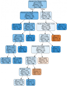
In the call to export_graphviz we specify class names:

export_graphviz(tree, out_file=f, feature_names=feature_names, filled=True, rounded=True, class_names=[“Low”, “High”] )

The rest of the code is the same as in previous post for regression tree.

Here is the python computer code:


# -*- coding: utf-8 -*-


import pandas as pd
from sklearn.cross_validation import train_test_split
from sklearn.tree import DecisionTreeClassifier
import subprocess

from sklearn.tree import  export_graphviz


def visualize_tree(tree, feature_names):
    
    with open("dt.dot", 'w') as f:
        
        export_graphviz(tree, out_file=f, feature_names=feature_names,  filled=True, rounded=True, class_names=["Low", "High"] )

    command = ["C:\\Program Files (x86)\\Graphviz2.38\\bin\\dot.exe", "-Tpng", "C:\\Users\\Owner\\Desktop\\A\\Python_2016_A\\dt.dot", "-o", "dt.png"]
    
       
    try:
        subprocess.check_call(command)
    except:
        exit("Could not run dot, ie graphviz, to "
             "produce visualization")
    
data = pd.read_csv('adwords_data.csv', sep= ',' , header = 1)


X = data.values[:, [3,17,18,19,20,21,22]]
Y = data.values[:,8]

                           
X_train, X_test, y_train, y_test = train_test_split( X, Y, test_size = 0.3, random_state = 100)                           
                           
clf_gini = DecisionTreeClassifier(criterion = "gini", random_state = 100, 
                               max_depth=8, min_samples_leaf=4)
clf_gini.fit(X_train, y_train)   


visualize_tree(clf_gini, ["Words in Key Phrase", "AdSense",	"Mortgage",	"Money",	"loan", 	"lawyer", 	"attorney"])


Decision Tree (partial view)

References
1. Decision tree Wikipedia
2. MLlib – Decision Trees
3. Visual analysis of AdWords data: a primer
4. 2 main differences between classification and regression trees
5. strings as features in decision tree/random forest
6. Decision Trees with scikit-learn
7. Classification: Basic Concepts, Decision Trees, and Model Evaluation
8. Understanding decision tree output from export_graphviz
9. Building Decision Trees in Python
10. Converting Categorical Text Variable into Binary Variables


Building Decision Trees in Python

A decision tree is a decision support tool that uses a tree-like graph or model of decisions and their possible consequences, including chance event outcomes, resource costs, and utility. It is one way to display an algorithm.
Decision trees are commonly used in operations research, specifically in decision analysis, to help identify a strategy most likely to reach a goal, but are also a popular tool in machine learning. [1]

Decision trees are widely used since they are easy to interpret, handle categorical features, extend to the multiclass classification setting, do not require feature scaling, and are able to capture non-linearities and feature interactions. [2] Decision trees are also one of the most widely used predictive analytics techniques.

Recently I decided to build python code for decision tree for AdWords data. This was motivated by the post [3] about visual analytics used for AdWords dataset. Below are the main components that I used for implementing decision tree.

Dataset
AdWords dataset – the dataset was obtained on Internet. Below is the table with few rows to show data. Only the columns that were used for decision tree, are shown in the table.

Keyword Number of words CPC Clicks CTR Cost Impressions
car insurance premium 3 176 7 0.012 1399 484
AdSense data 2 119 13 0.025 1061 466

The following independent variables were selected:
Number of words in keyword phrase – this column was added based on the keyword phrase column.
CTR – click through rate

For the dependent variable it was selected CPC – Average Cost per Click.

Python Module
As the dependent variable is numeric and continuos, the regression decision tree from python module sklearn.tree was used in the script:
from sklearn.tree import DecisionTreeRegressor

In sklearn.tree Decision Trees (DTs) are a non-parametric supervised learning method used for classification and regression. The goal is to create a model that predicts the value of a target variable by learning simple decision rules inferred from the data features. [5]

Visualization
For visualization of decision tree graphviz was installed. “Graphviz is open source graph visualization software. Graph visualization is a way of representing structural information as diagrams of abstract graphs and networks. It has important applications in networking, bioinformatics, software engineering, database and web design, machine learning, and in visual interfaces for other technical domains.”

Python Script
The created code consisted of the following steps:
reading data from csv data file
selecting needed columns
splitting dataset for testing and training
initializing DecisionTreeRegressor
visualizing decision tree via function. Note that the path to Graphviz are specified inside of scripts.

Decision tree and Python code are shown below. Online resources used for this post are provided in the reference section.

Decision Tree
Decision Tree

Python computer code:


# -*- coding: utf-8 -*-

import pandas as pd
from sklearn.cross_validation import train_test_split
from sklearn.tree import DecisionTreeRegressor


import subprocess

from sklearn.tree import  export_graphviz


def visualize_tree(tree, feature_names):
    
    with open("dt.dot", 'w') as f:
        
        export_graphviz(tree, out_file=f, feature_names=feature_names,  filled=True, rounded=True )

    command = ["C:\\Program Files (x86)\\Graphviz2.38\\bin\\dot.exe", "-Tpng", "C:\\Users\\Owner\\Desktop\\A\\Python_2016_A\\dt.dot", "-o", "dt.png"]
    
        
    try:
        subprocess.check_call(command)
    except:
        exit("Could not run dot, ie graphviz, to "
             "produce visualization")
    
data = pd.read_csv('adwords_data.csv', sep= ',' , header = 1)


X = data.values[:, [3,13]]
Y = data.values[:,11]

                       
X_train, X_test, y_train, y_test = train_test_split( X, Y, test_size = 0.3, random_state = 100)                           
                           
clf = DecisionTreeRegressor( random_state = 100,
                               max_depth=3, min_samples_leaf=4)
clf.fit(X_train, y_train)   


visualize_tree(clf, ["Words in Key Phrase", "CTR"])

References
1. Decision tree Wikipedia
2. MLlib – Decision Trees
3. Visual analysis of AdWords data: a primer
4. Decision trees in python with scikit_learn and pandas
5. Decision Tree
6. Graphviz – Graph Visualization Software