In the previous post Reinforcement Learning Example for Planning Tasks Using Q Learning and Dyna-Q we applied Dyna-Q algorithm for planning of actions to complete tasks. This problem can be viewed as resource allocation task. In this post we will use reinforcement learning python DQN (Deep Q-network) for the same problem. In case you did not read previous post the problem is described below.
The Problem
Given some goals (projects to complete) and set of actions (number of hours to put for each project per day) we are interesting to know what action we need to take (how many hours to put per project on each day) in order to get the best result in the end (we have reward for completion project in time).
So we are trying to allocate resource (time) for each project for each day in such way that it produces maximum reward in the end of given period. We have reward data and time needed to complete for each project.
The diagram of one of possible path would look like this:
Planning Diagram
On this diagram the green indicates path that produces the max reward 13 as the agent was able to complete both goals.
Deep Q-Network
Deep Q-Networks, abbreviated DQN, use deep neural networks as function approximation of the
action-value function q(s, a). The input of the artificial neural network used is the state and the output is the estimated q-values of the state-action pairs.
In DQN the replay memory simply stores the transitions such that they can be used at later times. By sampling transitions from the replay memory the network increases its ability to generalize. This also allows the network to predict the correct values in states which might be visited less frequently when the agent’s strategy gets better.
Also we add a second network, a target network, which is a copy of the first network, which we call the training network. The target network is only used to predict the value of taking the optimal action from s0 when updating the training network. The target network is updated with a certain frequency by copying the weights from the training network. This prevents instability when s and s0 are equal or even similar which is often the case. [1]
Solution
The code here is based on DQN with Tensorflow for maze problem[2] and previous code for Dyna-Q mentioned in the beginning of the post. It has 2 modules for programming environment and Reinforcement Learning Tensorflow DQN algorithm. Additionally it has main module which run the loop with episodes.
To run this reinforcement learning example you can use reinforcement learning python source code from the links below:
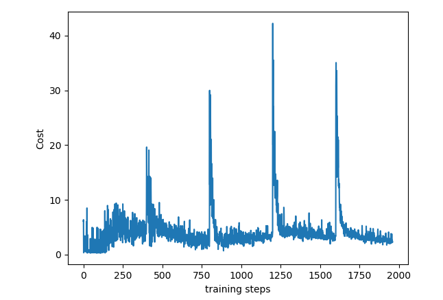
Below are charts obtained from running program. Performance (achieving max possible reward) with DQN is a little higher (but not significantly) than with Dyna-Q example on the same problem.
In this post we will learn how to use sentiment analysis with API python from paralleldots.com. We will look at running this API from python environment on laptop and also in web application environment with python Django on pythonanywhere hosting site.
In the one of previous post we set python Django project for chatbot. Here we will add file to this environment. Setting the chatbot files from previous project is not necessary. We just need folder structure.
Thus in this post we will reuse and extend some python Django knowledge that we got in the previous post. We will learn how to pass parameters from user form to server and back to user form, how to serve images, how to have logic block in web template.
ParrallelDots [1] provides several machine learning APIs such as named entity recognition (NER), intent identification, text classification and sentiment analysis. In this post we will explore sentiment analysis API and how it can be deployed on web server with Diango python.
Running Text Analysis API Locally
First we need install the library:
pip install paralleldots
We need also obtain key. It is free and no credit card required.
Now we run code as below
import paralleldots
paralleldots.set_api_key("XXXXXXXXXXX")

# for single sentence
text="the day is very nice"
lang_code="en"
response=paralleldots.sentiment(text,lang_code)

print(response)
print (response['sentiment'])
print (response['code'])
print (response['probabilities']['positive'])
print (response['probabilities']['negative'])
print (response['probabilities']['neutral'])


# for multiple sentence as array
text=["the day is very nice,the day is very good,this is the best day"]
response=paralleldots.batch_sentiment(text)
print(response)

Output:
{'probabilities': {'negative': 0.001, 'neutral': 0.002, 'positive': 0.997}, 'sentiment': 'positive', 'code': 200}
positive
200
0.997
0.001
0.002
{'sentiment': [{'negative': 0.0, 'neutral': 0.001, 'positive': 0.999}], 'code': 200}
This is very simple. Now we will deploy on web hosting site with python Django.
Deploying API on Web Hosting Site
Here we will build web form. Using this web form user can enter some text which will be passed to semantic analysis API. The result of analysis will be passed back to user and image will be shown based on result of sentiment analysis.
First we need install paralleldots library. To install the paralleldots module for Python 3.6, we’d run this in a Bash console (not in a Python one): [2]
pip3.6 install –user paralleldots
Note it is two dashes before user.
Now create or update the following files:
views.py
In this file we are getting user input from web form and sending it to API. Based on sentiment output from API we select image filename.
my_template_img.html
Create new file my_template_img.html This file will have web input form for user to enter some text. We have also if statement here because we do not want display image when the form is just opened and no submission is done.
urls.py
This file is located under /home/username/projectname/projectname. Add import line to this file and also include pattern for do_sentiment_analysis:
Now when all is set, just access link. In case we use pythonanywhere it will be: http://username.pythonanywhere.com/do_sentiment_analysis/
Enter some text into text box and click Submit. We will see the output of API for sentiment analysis result and image based on this sentiment. Below are some screenshots.
Conclusion
We integrated machine learning sentiment analysis API from parallelDots into our python Diango web environment. We built web user input form that can send data to this API and receive output from API to show it to user. While building this we learned some Django things:
how to pass parameters from user form to server and back to user form,
how to serve images,
how to have logic block in web template.
We can build now different web applications that would use API service from ParallelDots. And we are able now integrate emotion analysis from text into our website.
Doing different activities we often are interesting how they impact each other. For example, if we visit different links on Internet, we might want to know how this action impacts our motivation for doing some specific things. In other words we are interesting in inferring importance of causes for effects from our daily activities data.
In this post we will look at few ways to detect relationships between actions and results using machine learning algorithms and python.
Our data example will be artificial dataset consisting of 2 columns: URL and Y.
URL is our action and we want to know how it impacts on Y. URL can be link0, link1, link2 wich means links visited, and Y can be 0 or 1, 0 means we did not got motivated, and 1 means we got motivated.
The first thing we do hot-encoding link0, link1, link3 in 0,1 and we will get 3 columns as below. Sample of data after one hot encoding
So we have now 3 features, each for each URL. Here is the code how to do hot-encoding to prepare our data for cause and effect analysis.
Now we can apply feature extraction algorithm. It allows us select features according to the k highest scores.
# feature extraction
test = SelectKBest(score_func=chi2, k="all")
fit = test.fit(X, Y)
# summarize scores
numpy.set_printoptions(precision=3)
print ("scores:")
print(fit.scores_)

for i in range (len(fit.scores_)):
    print ( str(dataframe.columns.values[i]) + "    " + str(fit.scores_[i]))
features = fit.transform(X)

print (list(dataframe))

numpy.set_printoptions(threshold=numpy.inf)


scores:
[11.475  0.142 15.527]
URL_link0    11.475409836065575
URL_link1    0.14227166276346598
URL_link2    15.526957539965377
['URL_link0', 'URL_link1', 'URL_link2', 'Y']


Another algorithm that we can use is <strong>ExtraTreesClassifier</strong> from python machine learning library sklearn.


from sklearn.ensemble import ExtraTreesClassifier
from sklearn.feature_selection import SelectFromModel

clf = ExtraTreesClassifier()
clf = clf.fit(X, Y)
print (clf.feature_importances_)
model = SelectFromModel(clf, prefit=True)
X_new = model.transform(X)
print (X_new.shape)

#output
#[0.424 0.041 0.536]
#(150, 2)
The above two machine learning algorithms helped us to estimate the importance of our features (or actions) for our Y variable. In both cases URL_link2 got highest score.
There exist other methods. I would love to hear what methods do you use and for what datasets and/or problems. Also feel free to provide feedback or comments or any questions.
Can sweet food affect our mood? A friend of mine was interesting if some of his minor mood changes are caused by sugar intake from sweets like cookies. He collected and provided records and in this post we will use correlation data analysis with python pandas dataframes to check the connection between food and mood. We will create python script for this task.
From internet resources we can confirm that relationship between how we feel and what we eat exists.[1] Sweet food is not recommended to eat as fluctuations in blood sugar cause mood swings, lack of energy [2]. The information about chocolate is however contradictory. Chocolate affects us both negatively and positively.[3] But chocolate has also sugar.
What if we eat only small amount of sweets and not each day – is there still any connection and how strong is it? The machine learning data analysis can help us to investigate this.
The Problem
So in this post we will estimate correlation between sweet food and mood based on provided daily data. Correlation means association – more precisely it is a measure of the extent to which two variables are related. [4]
Data
The dataset has two columns, X and Y where: X is how much sweet food was taken on daily basis, on the scale 0 – 1 , 0 is nothing, 1 means a max value. Y is variation of mood from optimal state, on the scale 0 – 1 , 0 – means no variations or no defects, 1 means a max value.
Approach
If we calculate correlation between 2 columns of daily data we will get something around 0. However this would not show whole picture. Because the effect of the food might take action in a few days. The good or bad feeling can also stay for few days after the event that caused this feeling.
So we would need to take average data for several days for both X (looking back) and Y (looking forward). Here is the diagram that explains how data will be aggregated:
Changing the data – averaging
And here is how we can do this in the program:
1.for each day take average X data for last N days and take average Y data for M next days.
2.create a pandas dataframe which has now new moving averages for X and Y.
3.calculate correlation between new X and Y data
What should be N and M? We will use different values – from 1 to 14. And we will check what is the highest value for correlation.
Here is the python code to use pandas dataframe for calculating averages:
def get_data (df_pandas,k,z):

    x = np.zeros(df_pandas.shape[0])
    y = np.zeros(df_pandas.shape[0])

    new_df = pd.DataFrame() #creates a new dataframe that's empty
    for index, row in df_pandas.iterrows():

        x[index]=df_pandas.loc[index-k:index,'X'].mean()

        y[index]=df_pandas.loc[index:index+z,'Y'].mean()

    new_df=pd.concat([pd.DataFrame(x),pd.DataFrame(y)], "columns")
    new_df.columns = ['X', 'Y']

    return new_df
Correlation Data Analysis
For calculating correlation we use also pandas dataframe. Here is the code snipped for this:
for i in range (1,n):
    for j in range (1,m):

       data=get_data(df, i, j)
       corr_df.loc[i, j] = data['X'].corr(data['Y'])

print ("corr_df")
print (corr_df)
pandas.DataFrame.corr by default is calculating pearson correlation coefficient – it is the measure of the strength of the linear relationship between two variables. In our code we use this default option. [8]
Results
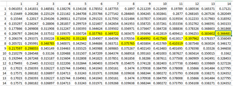
After calculating correlation coefficients we output data in the table format and plot results on heatmap using seaborn module. Below is the data output and the plot. The max value of correlation for each column is highlighted in yellow in the data table. Input data and full source code are available at [5],[6].
Correlation data between sweet food (taken in n days) and mood (in next m days)Correlation data between sweet food (taken in N days) and mood in the following M days, averaged
Conclusion
We performed correlation analysis between eating sweet food and mental health. And we confirmed that in our data example there is a moderate correlation (0.4). This correlation is showing up when we use moving averaging for 5 or 6 days. This corresponds with observation that swing mood may appear in several days, not on the same or next day after eating sweet food.
We also learned how we can estimate correlation between two time series variables X, Y.
Neural networks are among the most widely used machine learning techniques.[1] But neural network training and tuning multiple hyper-parameters takes time. I was recently building LSTM neural network for prediction for this post Machine Learning Stock Market Prediction with LSTM Keras and I learned some tricks that can save time. In this post you will find some techniques that helped me to do neural net training more efficiently.
1. Adjusting Graph To See All Details
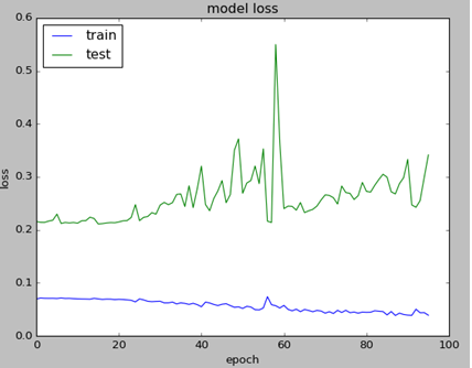
Sometimes validation loss is getting high value and this prevents from seeing other data on the chart. I added few lines of code to cut high values so you can see all details on chart.
import matplotlib.pyplot as plt
import matplotlib.ticker as mtick

T=25
history_val_loss=[]

for x in history.history['val_loss']:
      if x >= T:
             history_val_loss.append (T)
      else:
             history_val_loss.append( x )

plt.figure(6)
plt.plot(history.history['loss'])
plt.plot(history_val_loss)
plt.title('model loss adjusted')
plt.ylabel('loss')
plt.xlabel('epoch')
plt.legend(['train', 'test'], loc='upper left')
Below is the example of charts. Left graph is not showing any details except high value point because of the scale. Note that graphs are obtained from different tests. LSTM NN Training Value Loss Charts with High Number and Adjusted
2. Early Stopping
Early stopping is allowing to save time on not running tests when a monitored quantity has stopped improving. Here is how it can be coded:
Here is what arguments mean per Keras documentation [2].
min_delta: minimum change in the monitored quantity to qualify as an improvement, i.e. an absolute change of less than min_delta, will count as no improvement.
patience: number of epochs with no improvement after which training will be stopped.
verbose: verbosity mode.
mode: one of {auto, min, max}. In min mode, training will stop when the quantity monitored has stopped decreasing; in max mode it will stop when the quantity monitored has stopped increasing; in auto mode, the direction is automatically inferred from the name of the monitored quantity.
3. Weight Regularization
Weight regularizer can be used to regularize neural net weights. Here is the example.
I found that beta_1=0.89 performed better then suggested 0.91 or other tested values.
5. Rolling Window Size
Rolling window (in case we use it) also can impact on performance. Too small or too big will drive higher validation loss. Below are charts for different window size (N=4,8,16,18, from left to right). In this case the optimal value was 16 which resulted in 81% accuracy.
LSTM Neural Net Loss Charts with Different N
I hope you enjoyed this post on different techniques for tuning hyper parameters. If you have any tips or anything else to add, please leave a comment below in the comment box.
Below is the full source code:
import numpy as np
import pandas as pd
from sklearn import preprocessing

import matplotlib.pyplot as plt
import matplotlib.ticker as mtick

from keras.regularizers import L1L2

fname="C:\\Users\\stock data\\GM.csv"
data_csv = pd.read_csv (fname)

#how many data we will use
# (should not be more than dataset length )
data_to_use= 150

# number of training data
# should be less than data_to_use
train_end =120


total_data=len(data_csv)

#most recent data is in the end
#so need offset
start=total_data - data_to_use


yt = data_csv.iloc [start:total_data ,4]    #Close price
yt_ = yt.shift (-1)

print (yt_)

data = pd.concat ([yt, yt_], axis =1)
data. columns = ['yt', 'yt_']


N=16
cols =['yt']
for i in range (N):

    data['yt'+str(i)] = list(yt.shift(i+1))
    cols.append ('yt'+str(i))

data = data.dropna()
data_original = data
data=data.diff()
data = data.dropna()


# target variable - closed price
# after shifting
y = data ['yt_']
x = data [cols]


scaler_x = preprocessing.MinMaxScaler ( feature_range =( -1, 1))
x = np. array (x).reshape ((len( x) ,len(cols)))
x = scaler_x.fit_transform (x)

scaler_y = preprocessing. MinMaxScaler ( feature_range =( -1, 1))
y = np.array (y).reshape ((len( y), 1))
y = scaler_y.fit_transform (y)


x_train = x [0: train_end,]
x_test = x[ train_end +1:len(x),]
y_train = y [0: train_end]
y_test = y[ train_end +1:len(y)]

x_train = x_train.reshape (x_train. shape + (1,))
x_test = x_test.reshape (x_test. shape + (1,))

from keras.models import Sequential
from keras.layers.core import Dense
from keras.layers.recurrent import LSTM
from keras.layers import  Dropout
from keras import optimizers

from numpy.random import seed
seed(1)
from tensorflow import set_random_seed
set_random_seed(2)

from keras import regularizers

from keras.callbacks import EarlyStopping


earlystop = EarlyStopping(monitor='val_loss', min_delta=0.0001, patience=80,  verbose=1, mode='min')
callbacks_list = [earlystop]

model = Sequential ()
model.add (LSTM ( 400,  activation = 'relu', inner_activation = 'hard_sigmoid' , bias_regularizer=L1L2(l1=0.01, l2=0.01),  input_shape =(len(cols), 1), return_sequences = False ))
model.add(Dropout(0.3))
model.add (Dense (output_dim =1, activation = 'linear', activity_regularizer=regularizers.l1(0.01)))
adam=optimizers.Adam(lr=0.01, beta_1=0.89, beta_2=0.999, epsilon=None, decay=0.0, amsgrad=True)
model.compile (loss ="mean_squared_error" , optimizer = "adam")
history=model.fit (x_train, y_train, batch_size =1, nb_epoch =1000, shuffle = False, validation_split=0.15, callbacks=callbacks_list)


y_train_back=scaler_y.inverse_transform (np. array (y_train). reshape ((len( y_train), 1)))
plt.figure(1)
plt.plot (y_train_back)


fmt = '%.1f'
tick = mtick.FormatStrFormatter(fmt)
ax = plt.axes()
ax.yaxis.set_major_formatter(tick)
print (model.summary())

print(history.history.keys())

T=25
history_val_loss=[]

for x in history.history['val_loss']:
      if x >= T:
             history_val_loss.append (T)
      else:
             history_val_loss.append( x )


plt.figure(2)
plt.plot(history.history['loss'])
plt.plot(history.history['val_loss'])
plt.title('model loss')
plt.ylabel('loss')
plt.xlabel('epoch')
plt.legend(['train', 'test'], loc='upper left')
fmt = '%.1f'
tick = mtick.FormatStrFormatter(fmt)
ax = plt.axes()
ax.yaxis.set_major_formatter(tick)


plt.figure(6)
plt.plot(history.history['loss'])
plt.plot(history_val_loss)
plt.title('model loss adjusted')
plt.ylabel('loss')
plt.xlabel('epoch')
plt.legend(['train', 'test'], loc='upper left')


score_train = model.evaluate (x_train, y_train, batch_size =1)
score_test = model.evaluate (x_test, y_test, batch_size =1)
print (" in train MSE = ", round( score_train ,4))
print (" in test MSE = ", score_test )

pred1 = model.predict (x_test)
pred1 = scaler_y.inverse_transform (np. array (pred1). reshape ((len( pred1), 1)))

prediction_data = pred1[-1]
model.summary()
print ("Inputs: {}".format(model.input_shape))
print ("Outputs: {}".format(model.output_shape))
print ("Actual input: {}".format(x_test.shape))
print ("Actual output: {}".format(y_test.shape))

print ("prediction data:")
print (prediction_data)

y_test = scaler_y.inverse_transform (np. array (y_test). reshape ((len( y_test), 1)))
print ("y_test:")
print (y_test)

act_data = np.array([row[0] for row in y_test])

fmt = '%.1f'
tick = mtick.FormatStrFormatter(fmt)
ax = plt.axes()
ax.yaxis.set_major_formatter(tick)

plt.figure(3)
plt.plot( y_test, label="actual")
plt.plot(pred1, label="predictions")

print ("act_data:")
print (act_data)

print ("pred1:")
print (pred1)

plt.legend(loc='upper center', bbox_to_anchor=(0.5, -0.05),
          fancybox=True, shadow=True, ncol=2)


fmt = '$%.1f'
tick = mtick.FormatStrFormatter(fmt)
ax = plt.axes()
ax.yaxis.set_major_formatter(tick)

def moving_test_window_preds(n_future_preds):

    ''' n_future_preds - Represents the number of future predictions we want to make
                         This coincides with the number of windows that we will move forward
                         on the test data
    '''
    preds_moving = []                                    # Store the prediction made on each test window
    moving_test_window = [x_test[0,:].tolist()]          # First test window
    moving_test_window = np.array(moving_test_window)

    for i in range(n_future_preds):


        preds_one_step = model.predict(moving_test_window)
        preds_moving.append(preds_one_step[0,0])

        preds_one_step = preds_one_step.reshape(1,1,1)
        moving_test_window = np.concatenate((moving_test_window[:,1:,:], preds_one_step), axis=1) # new moving test window, where the first element from the window has been removed and the prediction  has been appended to the end


    print ("pred moving before scaling:")
    print (preds_moving)

    preds_moving = scaler_y.inverse_transform((np.array(preds_moving)).reshape(-1, 1))

    print ("pred moving after scaling:")
    print (preds_moving)
    return preds_moving

print ("do moving test predictions for next 22 days:")
preds_moving = moving_test_window_preds(22)


count_correct=0
error =0
for i in range (len(y_test)):
    error=error + ((y_test[i]-preds_moving[i])**2) / y_test[i]


    if y_test[i] >=0 and preds_moving[i] >=0 :
        count_correct=count_correct+1
    if y_test[i] < 0 and preds_moving[i] < 0 :
        count_correct=count_correct+1

accuracy_in_change =  count_correct / (len(y_test) )

plt.figure(4)
plt.title("Forecast vs Actual, (data is differenced)")
plt.plot(preds_moving, label="predictions")
plt.plot(y_test, label="actual")
plt.legend(loc='upper center', bbox_to_anchor=(0.5, -0.05),
          fancybox=True, shadow=True, ncol=2)


print ("accuracy_in_change:")
print (accuracy_in_change)

ind=data_original.index.values[0] + data_original.shape[0] -len(y_test)-1
prev_starting_price = data_original.loc[ind,"yt_"]
preds_moving_before_diff =  [0 for x in range(len(preds_moving))]

for i in range (len(preds_moving)):
    if (i==0):
        preds_moving_before_diff[i]=prev_starting_price + preds_moving[i]
    else:
        preds_moving_before_diff[i]=preds_moving_before_diff[i-1]+preds_moving[i]


y_test_before_diff = [0 for x in range(len(y_test))]

for i in range (len(y_test)):
    if (i==0):
        y_test_before_diff[i]=prev_starting_price + y_test[i]
    else:
        y_test_before_diff[i]=y_test_before_diff[i-1]+y_test[i]


plt.figure(5)
plt.title("Forecast vs Actual (non differenced data)")
plt.plot(preds_moving_before_diff, label="predictions")
plt.plot(y_test_before_diff, label="actual")
plt.legend(loc='upper center', bbox_to_anchor=(0.5, -0.05),
          fancybox=True, shadow=True, ncol=2)
plt.show()


You must be logged in to post a comment.