owygs156

In the post Bitcoin trading with Python — Bollinger Bands strategy analysis the author reported 34% returns over the initial investment on back test. Does it work all the time? Is it the best strategy?

Let us use backtrader platform and compare several strategies just for buy signal. Backtrader is a feature-rich Python framework for backtesting and trading. Backtrader allows you to focus on writing reusable trading strategies, indicators and analyzers instead of having to spend time building infrastructure.

We will use the following strategies:

Crossover – based on two simple moving averages (SMA) with periods 10 and 30 days. Buy if fast SMA line crosses slow to the upside.

Consecutive 2 prices (Simple1) – Buy if two consecutive prices are decreasing – if current price is less than previous price and previous price is also less than previous price

  if self.dataclose[0] < self.dataclose[-1]:
                    if self.dataclose[-1] < self.dataclose[-2]:
                         self.log('BUY CREATE {0:8.2f}'.format(self.dataclose[0]))
                         self.order = self.buy()

Consecutive 4 prices (Simple2) – Buy if within 4 price windows we have decrease more than 5% of original price between any two prices from this window:

   if tr_str == "simple2":
            # since there is no order pending, are we in the market?    
            if not self.position: # not in the market
                if (self.dataclose[0] - self.dataclose[-1]) < -0.05*self.dataclose[0] or (self.dataclose[0] - self.dataclose[-2]) < -0.05*self.dataclose[0] or (self.dataclose[0] - self.dataclose[-3]) < -0.05*self.dataclose[0] or (self.dataclose[0] - self.dataclose[-4]) < -0.05*self.dataclose[0]:
                    #if self.dataclose[-1] < self.dataclose[-2]:
                        self.log('BUY CREATE {0:8.2f}'.format(self.dataclose[0]))
                        self.order = self.buy() 

Bollinger Bands – Buy when the price cross the bottom band.

  if self.data.close < self.boll.lines.bot:
                self.log('BUY CREATE {0:8.2f}'.format(self.dataclose[0]))
                self.order = self.buy()     

Our starting asset value is 10000. We use daily prices.
After running above strategies we get results like below:

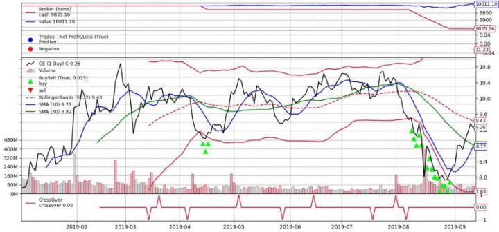
Final Vaues for Strategies

cross 9999.06  
simple1 9999.31  
simple2 9999.91  
BB 10011.099999999999  

Thus we see that Bollinger Band looks more promising comparing with other strategies that we tried. However we did not do any optimization – using different parameters to improve performance of strategy. We learned how to set different strategies with backtrader and got understanding how to issue buy signal. Below you can find full source code.

# -*- coding: utf-8 -*-
import matplotlib
import matplotlib.pyplot as plt

from datetime import datetime
import backtrader as bt

matplotlib.use('Qt5Agg')
plt.switch_backend('Qt5Agg')

# Create a subclass of Strategy to define the indicators and logic
class SmaCross(bt.Strategy):
    # parameters which are configurable for the strategy
    params = dict(
        pfast=10,  # period for the fast moving average
        pslow=30,   # period for the slow moving average
    )
     params['tr_strategy'] = None

    def __init__(self):
          
        self.boll = bt.indicators.BollingerBands(period=50, devfactor=2)
        self.dataclose= self.datas[0].close    # Keep a reference to 
        self.sma1 = bt.ind.SMA(period=self.p.pfast)  # fast moving average
        self.sma2 = bt.ind.SMA(period=self.p.pslow)  # slow moving average
        self.crossover = bt.ind.CrossOver(self.sma1, self.sma2)  # crossover signal
        self.tr_strategy = self.params.tr_strategy

    def next(self, strategy_type=""):
        tr_str = self.tr_strategy
        print (self.tr_strategy)
       
        # Log the closing prices of the series
        self.log("Close, {0:8.2f} ".format(self.dataclose[0]))
        self.log('sma1, {0:8.2f}'.format(self.sma1[0]))
        
        if tr_str == "cross":
            if not self.position:  # not in the market
                if self.crossover > 0:  # if fast crosses slow to the upside
                    self.buy()  # enter long

              
        if tr_str == "simple1":
          
            if not self.position: # not in the market
                if self.dataclose[0] < self.dataclose[-1]:
                    if self.dataclose[-1] < self.dataclose[-2]:
                        self.log('BUY CREATE {0:8.2f}'.format(self.dataclose[0]))
                        self.order = self.buy()
                        
        if tr_str == "simple2":
           
            if not self.position: # not in the market
                if (self.dataclose[0] - self.dataclose[-1]) < -0.05*self.dataclose[0] or (self.dataclose[0] - self.dataclose[-2]) < -0.05*self.dataclose[0] or (self.dataclose[0] - self.dataclose[-3]) < -0.05*self.dataclose[0] or (self.dataclose[0] - self.dataclose[-4]) < -0.05*self.dataclose[0]:
                  
                        self.log('BUY CREATE {0:8.2f}'.format(self.dataclose[0]))
                        self.order = self.buy()                
                        
        if tr_str == "BB":
            #if self.data.close > self.boll.lines.top:
            #self.sell(exectype=bt.Order.Stop, price=self.boll.lines.top[0], size=self.p.size)
            if self.data.close < self.boll.lines.bot:
                self.log('BUY CREATE {0:8.2f}'.format(self.dataclose[0]))
                self.order = self.buy()     
                
        print('Current Portfolio Value: %.2f' % cerebro.broker.getvalue())            
        
    def log(self, txt, dt=None):
        # Logging function for the strategy.  'txt' is the statement and 'dt' can be used to specify a specific datetime
        dt = dt or self.datas[0].datetime.date(0)
        print('{0},{1}'.format(dt.isoformat(),txt))
     
        
    def notify_trade(self,trade):
        if not trade.isclosed:
            return
        
        self.log('OPERATION PROFIT, GROSS {0:8.2f}, NET {1:8.2f}'.format(
            trade.pnl, trade.pnlcomm))    
 
        
strategy_final_values=[0,0,0,0]
strategies = ["cross", "simple1", "simple2", "BB"]


for tr_strategy in strategies:         

    cerebro = bt.Cerebro()  # create a "Cerebro" engine instance
       
    data = bt.feeds.GenericCSVData(
        dataname='GE.csv',
    
        fromdate=datetime(2019, 1, 1),
        todate=datetime(2019, 9, 13),
  
        nullvalue=0.0,
    
        dtformat=('%Y-%m-%d'),
  
        datetime=0,
        high=2,
        low=3,
        open=1,
        close=4,
        adjclose=5,
        volume=6,
        openinterest=-1
      
    )
    

    print ("data")
    print (data )
    cerebro.adddata(data)  # Add the data feed

    # Print out the starting conditions
    print('Starting Portfolio Value: %.2f' % cerebro.broker.getvalue())
    
    
    cerebro.addstrategy(SmaCross, tr_strategy=tr_strategy)  # Add the trading strategy
    result=cerebro.run()  # run it all
    figure=cerebro.plot(iplot=False)[0][0]  
    figure.savefig('example.png')
    
    # Print out the final result
    print('Final Portfolio Value: %.2f' % cerebro.broker.getvalue())
    ind=strategies.index(tr_strategy)
    strategy_final_values[ind] = cerebro.broker.getvalue()
    
print ("Final Vaues for Strategies")
for tr_strategy in strategies: 
    ind=strategies.index(tr_strategy)
    print ("{} {}  ". format(tr_strategy, strategy_final_values[ind]))     
 

References
1. Backtrader
2. BackTrader Documentation – Quickstart
3. Backtrader: Bollinger Mean Reversion Strategy
4. Bitcoin trading with Python — Bollinger Bands strategy analysis