Building Decision Trees in Python – Handling Categorical Data

In the post Building Decision Trees in Python we looked at the decision tree with numerical continuous dependent variable. This type of decision trees can be called also regression tree.

But what if we need to use categorical dependent variable? It is still possible to create decision tree and in this post we will look how to create decision tree if dependent variable is categorical data. In this case the decision tree is called classification tree. Classification trees, as the name implies are used to separate the dataset into classes belonging to the response variable. [4] Classification is a typical problem that can be found in such fields as machine learning, predictive analytics, data mining.

Getting Data
For simplicity we will use the same dataset as before but will convert numerical target variable into categorical variable as we want build python code for decision tree with categorical dependent variable.
To convert dependent variable into categorical we use the following simple rule:
if CPC < 22 then CPC = "Low"
else CPC = “High”

For independent variables we will use “keyword” and “number of words” fields.
Keyword (usually it is several words) is a categorical variable. In general it is not the problem as in either case (regression or classification tree), the predictors or independent variables may be categorical or numeric. It is the target variable that determines the type of decision tree needed.[4]

However sklearn.tree (at least the version that is used here) does not support categorical independent variable. See discussion and suggestions on stack overflow [5]. To use independent categorical variable, we will code the categorical feature into multiple binary features. For example, we might code [‘red’,’green’,’blue’] with 3 columns, one for each category, having 1 when the category match and 0 otherwise. This is called one-hot-encoding, binary encoding, one-of-k-encoding or whatever. [5]

Below are shown few rows from the table data. We added 2 columns for categories “insurance”, “Adsense”. We actually have more categories and therefore we added more columns but this is not shown in the table.

For small dataset such conversion can be done manually. But we also created python script in the post Converting Categorical Text Variable into Binary Variables for this specific task. [10]

Keyword Number of words Insurance Adsense CTR Cost Cost (categorical)
car insurance premium 3 1 0 0.012 20 Low
AdSense data 2 0 1 0.025 1061 High

Building the Code
Now we need to build the code. The call for decision tree is looking like this:

clf_gini = DecisionTreeClassifier(criterion = “gini”, random_state = 100,
max_depth=8, min_samples_leaf=4)

we use here criterion Gini index for splitting data.
In the call to export_graphviz we specify class names:

export_graphviz(tree, out_file=f, feature_names=feature_names, filled=True, rounded=True, class_names=[“Low”, “High”] )

The rest of the code is the same as in previous post for regression tree.

Here is the python computer code:


# -*- coding: utf-8 -*-


import pandas as pd
from sklearn.cross_validation import train_test_split
from sklearn.tree import DecisionTreeClassifier
import subprocess

from sklearn.tree import  export_graphviz


def visualize_tree(tree, feature_names):
    
    with open("dt.dot", 'w') as f:
        
        export_graphviz(tree, out_file=f, feature_names=feature_names,  filled=True, rounded=True, class_names=["Low", "High"] )

    command = ["C:\\Program Files (x86)\\Graphviz2.38\\bin\\dot.exe", "-Tpng", "C:\\Users\\Owner\\Desktop\\A\\Python_2016_A\\dt.dot", "-o", "dt.png"]
    
       
    try:
        subprocess.check_call(command)
    except:
        exit("Could not run dot, ie graphviz, to "
             "produce visualization")
    
data = pd.read_csv('adwords_data.csv', sep= ',' , header = 1)


X = data.values[:, [3,17,18,19,20,21,22]]
Y = data.values[:,8]

                           
X_train, X_test, y_train, y_test = train_test_split( X, Y, test_size = 0.3, random_state = 100)                           
                           
clf_gini = DecisionTreeClassifier(criterion = "gini", random_state = 100, 
                               max_depth=8, min_samples_leaf=4)
clf_gini.fit(X_train, y_train)   


visualize_tree(clf_gini, ["Words in Key Phrase", "AdSense",	"Mortgage",	"Money",	"loan", 	"lawyer", 	"attorney"])
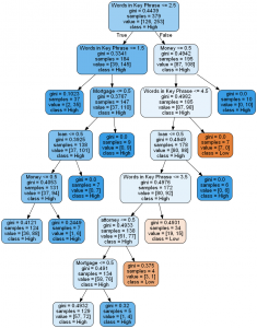

Decision Tree (partial view)

References
1. Decision tree Wikipedia
2. MLlib – Decision Trees
3. Visual analysis of AdWords data: a primer
4. 2 main differences between classification and regression trees
5. strings as features in decision tree/random forest
6. Decision Trees with scikit-learn
7. Classification: Basic Concepts, Decision Trees, and Model Evaluation
8. Understanding decision tree output from export_graphviz
9. Building Decision Trees in Python
10. Converting Categorical Text Variable into Binary Variables


Building Decision Trees in Python

A decision tree is a decision support tool that uses a tree-like graph or model of decisions and their possible consequences, including chance event outcomes, resource costs, and utility. It is one way to display an algorithm.
Decision trees are commonly used in operations research, specifically in decision analysis, to help identify a strategy most likely to reach a goal, but are also a popular tool in machine learning. [1]

Decision trees are widely used since they are easy to interpret, handle categorical features, extend to the multiclass classification setting, do not require feature scaling, and are able to capture non-linearities and feature interactions. [2] Decision trees are also one of the most widely used predictive analytics techniques.

Recently I decided to build python code for decision tree for AdWords data. This was motivated by the post [3] about visual analytics used for AdWords dataset. Below are the main components that I used for implementing decision tree.

Dataset
AdWords dataset – the dataset was obtained on Internet. Below is the table with few rows to show data. Only the columns that were used for decision tree, are shown in the table.

Keyword Number of words CPC Clicks CTR Cost Impressions
car insurance premium 3 176 7 0.012 1399 484
AdSense data 2 119 13 0.025 1061 466

The following independent variables were selected:
Number of words in keyword phrase – this column was added based on the keyword phrase column.
CTR – click through rate

For the dependent variable it was selected CPC – Average Cost per Click.

Python Module
As the dependent variable is numeric and continuos, the regression decision tree from python module sklearn.tree was used in the script:
from sklearn.tree import DecisionTreeRegressor

In sklearn.tree Decision Trees (DTs) are a non-parametric supervised learning method used for classification and regression. The goal is to create a model that predicts the value of a target variable by learning simple decision rules inferred from the data features. [5]

Visualization
For visualization of decision tree graphviz was installed. “Graphviz is open source graph visualization software. Graph visualization is a way of representing structural information as diagrams of abstract graphs and networks. It has important applications in networking, bioinformatics, software engineering, database and web design, machine learning, and in visual interfaces for other technical domains.”

Python Script
The created code consisted of the following steps:
reading data from csv data file
selecting needed columns
splitting dataset for testing and training
initializing DecisionTreeRegressor
visualizing decision tree via function. Note that the path to Graphviz are specified inside of scripts.

Decision tree and Python code are shown below. Online resources used for this post are provided in the reference section.

Decision Tree
Decision Tree

Python computer code:


# -*- coding: utf-8 -*-

import pandas as pd
from sklearn.cross_validation import train_test_split
from sklearn.tree import DecisionTreeRegressor


import subprocess

from sklearn.tree import  export_graphviz


def visualize_tree(tree, feature_names):
    
    with open("dt.dot", 'w') as f:
        
        export_graphviz(tree, out_file=f, feature_names=feature_names,  filled=True, rounded=True )

    command = ["C:\\Program Files (x86)\\Graphviz2.38\\bin\\dot.exe", "-Tpng", "C:\\Users\\Owner\\Desktop\\A\\Python_2016_A\\dt.dot", "-o", "dt.png"]
    
        
    try:
        subprocess.check_call(command)
    except:
        exit("Could not run dot, ie graphviz, to "
             "produce visualization")
    
data = pd.read_csv('adwords_data.csv', sep= ',' , header = 1)


X = data.values[:, [3,13]]
Y = data.values[:,11]

                       
X_train, X_test, y_train, y_test = train_test_split( X, Y, test_size = 0.3, random_state = 100)                           
                           
clf = DecisionTreeRegressor( random_state = 100,
                               max_depth=3, min_samples_leaf=4)
clf.fit(X_train, y_train)   


visualize_tree(clf, ["Words in Key Phrase", "CTR"])

References
1. Decision tree Wikipedia
2. MLlib – Decision Trees
3. Visual analysis of AdWords data: a primer
4. Decision trees in python with scikit_learn and pandas
5. Decision Tree
6. Graphviz – Graph Visualization Software


Iris Data Set – Normalized Data

On this page you can find normalized iris data set that was used in Iris Plant Classification Using Neural Network – Online Experiments with Normalization and Other Parameters. The data set is divided to training data set (141 records) and testing data set (9 records, 3 for each class). Class label is shown separately.

To calculate normalized data, the below table was built.

min 4.3 2 1 0.1
max 7.9 4.4 6.9 2.5
max-min 3.6 2.4 5.9 2.4

Here min, max and min-max are taken over the columns of iris data set which are:
1. sepal length in cm
2. sepal width in cm
3. petal length in cm
4. petal width in cm

Training data set:

0.083333333 0.458333333 0.084745763 0.041666667
0.194444444 0.666666667 0.06779661 0.041666667
0.305555556 0.791666667 0.118644068 0.125
0.083333333 0.583333333 0.06779661 0.083333333
0.194444444 0.583333333 0.084745763 0.041666667
0.027777778 0.375 0.06779661 0.041666667
0.166666667 0.458333333 0.084745763 0
0.305555556 0.708333333 0.084745763 0.041666667
0.138888889 0.583333333 0.101694915 0.041666667
0.138888889 0.416666667 0.06779661 0
0 0.416666667 0.016949153 0
0.416666667 0.833333333 0.033898305 0.041666667
0.388888889 1 0.084745763 0.125
0.305555556 0.791666667 0.050847458 0.125
0.222222222 0.625 0.06779661 0.083333333
0.388888889 0.75 0.118644068 0.083333333
0.222222222 0.75 0.084745763 0.083333333
0.305555556 0.583333333 0.118644068 0.041666667
0.222222222 0.708333333 0.084745763 0.125
0.083333333 0.666666667 0 0.041666667
0.222222222 0.541666667 0.118644068 0.166666667
0.138888889 0.583333333 0.152542373 0.041666667
0.194444444 0.416666667 0.101694915 0.041666667
0.194444444 0.583333333 0.101694915 0.125
0.25 0.625 0.084745763 0.041666667
0.25 0.583333333 0.06779661 0.041666667
0.111111111 0.5 0.101694915 0.041666667
0.138888889 0.458333333 0.101694915 0.041666667
0.305555556 0.583333333 0.084745763 0.125
0.25 0.875 0.084745763 0
0.333333333 0.916666667 0.06779661 0.041666667
0.166666667 0.458333333 0.084745763 0
0.194444444 0.5 0.033898305 0.041666667
0.333333333 0.625 0.050847458 0.041666667
0.166666667 0.458333333 0.084745763 0
0.027777778 0.416666667 0.050847458 0.041666667
0.222222222 0.583333333 0.084745763 0.041666667
0.194444444 0.625 0.050847458 0.083333333
0.055555556 0.125 0.050847458 0.083333333
0.027777778 0.5 0.050847458 0.041666667
0.194444444 0.625 0.101694915 0.208333333
0.222222222 0.75 0.152542373 0.125
0.138888889 0.416666667 0.06779661 0.083333333
0.222222222 0.75 0.101694915 0.041666667
0.083333333 0.5 0.06779661 0.041666667
0.277777778 0.708333333 0.084745763 0.041666667
0.194444444 0.541666667 0.06779661 0.041666667
0.333333333 0.125 0.508474576 0.5
0.611111111 0.333333333 0.610169492 0.583333333
0.388888889 0.333333333 0.593220339 0.5
0.555555556 0.541666667 0.627118644 0.625
0.166666667 0.166666667 0.389830508 0.375
0.638888889 0.375 0.610169492 0.5
0.25 0.291666667 0.491525424 0.541666667
0.194444444 0 0.423728814 0.375
0.444444444 0.416666667 0.542372881 0.583333333
0.472222222 0.083333333 0.508474576 0.375
0.5 0.375 0.627118644 0.541666667
0.361111111 0.375 0.440677966 0.5
0.666666667 0.458333333 0.576271186 0.541666667
0.361111111 0.416666667 0.593220339 0.583333333
0.416666667 0.291666667 0.525423729 0.375
0.527777778 0.083333333 0.593220339 0.583333333
0.361111111 0.208333333 0.491525424 0.416666667
0.444444444 0.5 0.644067797 0.708333333
0.5 0.333333333 0.508474576 0.5
0.555555556 0.208333333 0.661016949 0.583333333
0.5 0.333333333 0.627118644 0.458333333
0.583333333 0.375 0.559322034 0.5
0.638888889 0.416666667 0.576271186 0.541666667
0.694444444 0.333333333 0.644067797 0.541666667
0.666666667 0.416666667 0.677966102 0.666666667
0.472222222 0.375 0.593220339 0.583333333
0.388888889 0.25 0.423728814 0.375
0.333333333 0.166666667 0.474576271 0.416666667
0.333333333 0.166666667 0.457627119 0.375
0.416666667 0.291666667 0.491525424 0.458333333
0.472222222 0.291666667 0.694915254 0.625
0.305555556 0.416666667 0.593220339 0.583333333
0.472222222 0.583333333 0.593220339 0.625
0.666666667 0.458333333 0.627118644 0.583333333
0.555555556 0.125 0.576271186 0.5
0.361111111 0.416666667 0.525423729 0.5
0.333333333 0.208333333 0.508474576 0.5
0.333333333 0.25 0.576271186 0.458333333
0.5 0.416666667 0.610169492 0.541666667
0.416666667 0.25 0.508474576 0.458333333
0.194444444 0.125 0.389830508 0.375
0.361111111 0.291666667 0.542372881 0.5
0.388888889 0.416666667 0.542372881 0.458333333
0.388888889 0.375 0.542372881 0.5
0.527777778 0.375 0.559322034 0.5
0.222222222 0.208333333 0.338983051 0.416666667
0.388888889 0.333333333 0.525423729 0.5
0.555555556 0.541666667 0.847457627 1
0.416666667 0.291666667 0.694915254 0.75
0.777777778 0.416666667 0.830508475 0.833333333
0.555555556 0.375 0.779661017 0.708333333
0.611111111 0.416666667 0.813559322 0.875
0.916666667 0.416666667 0.949152542 0.833333333
0.166666667 0.208333333 0.593220339 0.666666667
0.833333333 0.375 0.898305085 0.708333333
0.666666667 0.208333333 0.813559322 0.708333333
0.805555556 0.666666667 0.86440678 1
0.611111111 0.5 0.694915254 0.791666667
0.583333333 0.291666667 0.728813559 0.75
0.694444444 0.416666667 0.762711864 0.833333333
0.388888889 0.208333333 0.677966102 0.791666667
0.416666667 0.333333333 0.694915254 0.958333333
0.583333333 0.5 0.728813559 0.916666667
0.611111111 0.416666667 0.762711864 0.708333333
0.944444444 0.75 0.966101695 0.875
0.944444444 0.25 1 0.916666667
0.472222222 0.083333333 0.677966102 0.583333333
0.722222222 0.5 0.796610169 0.916666667
0.361111111 0.333333333 0.661016949 0.791666667
0.944444444 0.333333333 0.966101695 0.791666667
0.555555556 0.291666667 0.661016949 0.708333333
0.666666667 0.541666667 0.796610169 0.833333333
0.805555556 0.5 0.847457627 0.708333333
0.527777778 0.333333333 0.644067797 0.708333333
0.5 0.416666667 0.661016949 0.708333333
0.583333333 0.333333333 0.779661017 0.833333333
0.805555556 0.416666667 0.813559322 0.625
0.861111111 0.333333333 0.86440678 0.75
1 0.75 0.915254237 0.791666667
0.583333333 0.333333333 0.779661017 0.875
0.555555556 0.333333333 0.694915254 0.583333333
0.5 0.25 0.779661017 0.541666667
0.944444444 0.416666667 0.86440678 0.916666667
0.555555556 0.583333333 0.779661017 0.958333333
0.583333333 0.458333333 0.762711864 0.708333333
0.472222222 0.416666667 0.644067797 0.708333333
0.722222222 0.458333333 0.745762712 0.833333333
0.666666667 0.458333333 0.779661017 0.958333333
0.722222222 0.458333333 0.694915254 0.916666667
0.416666667 0.291666667 0.694915254 0.75
0.694444444 0.5 0.830508475 0.916666667
0.666666667 0.541666667 0.796610169 1
0.666666667 0.416666667 0.711864407 0.916666667
0.555555556 0.208333333 0.677966102 0.75

Testing data set
0.222222222 0.625 0.06779661 0.041666667
0.166666667 0.416666667 0.06779661 0.041666667
0.111111111 0.5 0.050847458 0.041666667
0.75 0.5 0.627118644 0.541666667
0.583333333 0.5 0.593220339 0.583333333
0.722222222 0.458333333 0.661016949 0.583333333
0.444444444 0.416666667 0.694915254 0.708333333
0.611111111 0.416666667 0.711864407 0.791666667
0.527777778 0.583333333 0.745762712 0.916666667

Training data set – class label values

0
0
0
0
0
0
0
0
0
0
0
0
0
0
0
0
0
0
0
0
0
0
0
0
0
0
0
0
0
0
0
0
0
0
0
0
0
0
0
0
0
0
0
0
0
0
0
0.5
0.5
0.5
0.5
0.5
0.5
0.5
0.5
0.5
0.5
0.5
0.5
0.5
0.5
0.5
0.5
0.5
0.5
0.5
0.5
0.5
0.5
0.5
0.5
0.5
0.5
0.5
0.5
0.5
0.5
0.5
0.5
0.5
0.5
0.5
0.5
0.5
0.5
0.5
0.5
0.5
0.5
0.5
0.5
0.5
0.5
0.5
1
1
1
1
1
1
1
1
1
1
1
1
1
1
1
1
1
1
1
1
1
1
1
1
1
1
1
1
1
1
1
1
1
1
1
1
1
1
1
1
1
1
1
1
1
1
1

Testing data set – class label values
0
0
0
0.5
0.5
0.5
1
1
1


Iris Plant Classification Using Neural Network – Online Experiments with Normalization and Other Parameters

Do we need to normalize input data for neural network? How differently will be results from running normalized and non normalized data? This will be explored in the post using Online Machine Learning Algorithms tool for classification of iris data set with feed-forward neural network.

Feed-forward Neural Network
Feed-forward neural networks are commonly used for classification. In this example we choose feed-forward neural network with back propagation training and gradient descent optimization method.

Our neural network has one hidden layer. The number of neuron units in this hidden layer and learning rate can be set by user. We do not need to code neural network because we use online tool that is taking training, testing data, number of neurons in hidden layer and learning rate parameters as input.

The output from this tool is classification results for testing data set, neural network weights and deltas at different iterations.

Data Set
As mentioned above we use iris data set for data input to neural network. The data set contains 3 classes of 50 instances each, where each class refers to a type of iris plant. [1] We remove first 3 rows for each class and save for testing data set. Thus the input data set has 141 rows and testing data set has 9 rows.

Normalization
We run neural network first time without normalization of input data. Then we run neural network with normalized data.
We use min max normalization which can be described by formula [2]:
xij = (xij – colmmin) /(colmmax – colmmin)

Where
colmmin = minimum value of the column
colmmax = maximum value of the column
xij = x(data item) present at ithrow and jthcolumn

Normalization is applied to both X and Y, so the possible values for Y become 0, 05, 1
and X become like :
0.083333333 0.458333333 0.084745763 0.041666667

You can view normalized data at this link : Iris Data Set – Normalized Data

Online Tool
Once data is ready we can to load data to neural network and run classification. Here are the steps how to use online Machine Learning Algorithms tool:
1.Access the link Online Machine Learning Algorithms with feed-forward neural network.
2.Select algorithm and click Load parameters for this model.
3.Input the data that you want to run.
4.Click Run now.
5.Click results link
6.Click Refresh button on this new page, you maybe will need click few times untill you see data output.
7.Scroll to the bottom page to see calculations.
For more detailed instruction use this link: How to Run Online Machine Learning Algorithms Tool

Experiments
We do 4 experiments as shown in the table below: 1 without normalization, and 3 with normalization and various learning rate and number of neurons hidden. Results are shown in the same table and the error graph shown below under the table. When iris data set was inputted without normalization, the text label is changed to numerical variable with values -1,0,1 The result is not satisfying with needed accuracy level. So decision is made to normalize data using min max method.

Here is the sample result from the last experiment, with the lowest error. The learning rate is 0.1 and the number of hidden neurons is 36. The delta error in the end of training is 1.09.

[[ 0.00416852]
[ 0.01650389]
[ 0.01021347]
[ 0.43996485]
[ 0.50235484]
[ 0.58338683]
[ 0.80222148]
[ 0.92640374]
[ 0.93291573]]

Results

Norma
lization
Learn. Rate Hidden units # Correct Total Accuracy Delta Error
No

0.5 4 3 9 33% 9.7
Yes (Min Max)

0.5 4 8 9 89% 1.25
Yes (Min Max)

0.1 4 9 9 100% 1.19
Yes (Min Max)

0.1 36 9 9 100% 1.09

Conclusion
Normalization can make huge difference on results. Further improvements are posible by adjusting learning rate or number hidden units in the hidden layer.

References

1. Iris Data Set
2. AN APPROACH FOR IRIS PLANT CLASSIFICATION USING NEURAL NETWORK


Latent Dirichlet Allocation (LDA) with Python Script

In the previous posts [1],[2] few scripts for extracting web data were created. Combining these scripts, we will create now web crawling script with text mining functionality such as Latent Dirichlet Allocation (LDA).

In LDA, each document may be viewed as a mixture of various topics. Where each document is considered to have a set of topics that are assigned to it via LDA.
Thus Each document is assumed to be characterized by a particular set of topics. This is akin to the standard bag of words model assumption, and makes the individual words exchangeable. [3]

Our web crawling script consists of the following parts:

1. Extracting links. The input file with pages to use is opening and each page is visted and links are extracted from this page using urllib.request. The extracted links are saved in csv file.
2. Downloading text content. The file with extracted links is opening and each link is visited and data (such as useful content no navigation, no advertisemet, html, title), are extracted using newspaper python module. This is running inside of function extract (url). Additionally extracted text content from each link is saving into memory list for LDA analysis on next step.
3. Text analyzing with LDA. Here thee script is preparing text data, doing actual LDA and outputting some results. Term, topic and probability also are saving in the file.

Below are the figure for script flow and full python source code.

Program Flow Chart for Extracting Data from Web and Doing LDA

# -*- coding: utf-8 -*-
from newspaper import Article, Config
import os
import csv
import time

import urllib.request
import lxml.html
import re

from nltk.tokenize import RegexpTokenizer
from stop_words import get_stop_words
from nltk.stem.porter import PorterStemmer
from gensim import corpora      
import gensim


regex = re.compile(r'\d\d\d\d')

path="C:\\Users\\Owner\\Python_2016"

#urlsA.csv file has the links for extracting web pages to visit
filename = path + "\\" + "urlsA.csv" 
filename_urls_extracted= path + "\\" + "urls_extracted.csv"

def load_file(fn):
         start=0
         file_urls=[]       
         with open(fn, encoding="utf8" ) as f:
            csv_f = csv.reader(f)
            for i, row in enumerate(csv_f):
               if i >=  start  :
                 file_urls.append (row)
         return file_urls

def save_extracted_url (fn, row):
    
         if (os.path.isfile(fn)):
             m="a"
         else:
             m="w"
    
       
         with open(fn, m, encoding="utf8", newline='' ) as csvfile: 
             fieldnames = ['url']
             writer = csv.DictWriter(csvfile, fieldnames=fieldnames)
             if (m=="w"):
                 writer.writeheader()
             writer.writerow(row)

urlsA= load_file (filename)
print ("Staring navigate...")
for u in urlsA:
  print  (u[0]) 
  req = urllib.request.Request(u[0], headers={'User-Agent': 'Mozilla/5.0'})
  connection = urllib.request.urlopen(req)
  print ("connected")
  dom =  lxml.html.fromstring(connection.read())
  time.sleep( 7 )
  links=[]
  for link in dom.xpath('//a/@href'): 
     try:
       
        links.append (link)
     except :
        print ("EXCP" + link)
     
  selected_links = list(filter(regex.search, links))
  

  link_data={}  
  for link in selected_links:
         link_data['url'] = link
         save_extracted_url (filename_urls_extracted, link_data)


#urls.csv file has the links for extracting content
filename = path + "\\" + "urls.csv" 
#data_from_urls.csv is file where extracted data is saved
filename_out= path + "\\"  + "data_from_urls.csv"
#below is the file where visited urls are saved
filename_urls_visited = path + "\\" + "visited_urls.csv"

#load urls from file to memory
urls= load_file (filename)
visited_urls=load_file (filename_urls_visited)


def save_to_file (fn, row):
    
         if (os.path.isfile(fn)):
             m="a"
         else:
             m="w"
    
         
         with open(fn, m, encoding="utf8", newline='' ) as csvfile: 
             fieldnames = ['url','authors', 'title', 'text', 'summary', 'keywords', 'publish_date', 'image', 'N']
             writer = csv.DictWriter(csvfile, fieldnames=fieldnames)
             if (m=="w"):
                 writer.writeheader()
             writer.writerow(row)


def save_visited_url (fn, row):
    
         if (os.path.isfile(fn)):
             m="a"
         else:
             m="w"
    
       
         with open(fn, m, encoding="utf8", newline='' ) as csvfile: 
             fieldnames = ['url']
             writer = csv.DictWriter(csvfile, fieldnames=fieldnames)
             if (m=="w"):
                 writer.writeheader()
             writer.writerow(row)
        
#to save html to file we need to know prev. number of saved file
def get_last_number():
    path="C:\\Users\\Owner\\Desktop\\A\\Python_2016_A"             
   
    count=0
    for f in os.listdir(path):
       if f[-5:] == ".html":
            count=count+1
    return (count)    

         
config = Config()
config.keep_article_html = True


def extract(url):
    article = Article(url=url, config=config)
    article.download()
    time.sleep( 7 )
    article.parse()
    article.nlp()
    return dict(
        title=article.title,
        text=article.text,
        html=article.html,
        image=article.top_image,
        authors=article.authors,
        publish_date=article.publish_date,
        keywords=article.keywords,
        summary=article.summary,
    )


doc_set = []

for url in urls:
    newsp=extract (url[0])
    newsp['url'] = url
    
    next_number =  get_last_number()
    next_number = next_number + 1
    newsp['N'] = str(next_number)+ ".html"
    
    
    with open(str(next_number) + ".html", "w",  encoding='utf-8') as f:
	     f.write(newsp['html'])
    print ("HTML is saved to " + str(next_number)+ ".html")
   
    del newsp['html']
    
    u = {}
    u['url']=url
    doc_set.append (newsp['text'])
    save_to_file (filename_out, newsp)
    save_visited_url (filename_urls_visited, u)
    time.sleep( 4 )


tokenizer = RegexpTokenizer(r'\w+')
en_stop = get_stop_words('en')
p_stemmer = PorterStemmer()
    

texts = []

# loop through all documents
for i in doc_set:
    
   
    raw = i.lower()
    tokens = tokenizer.tokenize(raw)
   
    stopped_tokens = [i for i in tokens if not i in en_stop]
   
    stemmed_tokens = [p_stemmer.stem(i) for i in stopped_tokens]
    
   
    texts.append(stemmed_tokens)
    
num_topics = 2    

dictionary = corpora.Dictionary(texts)
    

corpus = [dictionary.doc2bow(text) for text in texts]
print (corpus)

# generate LDA model
ldamodel = gensim.models.ldamodel.LdaModel(corpus, num_topics=num_topics, id2word = dictionary, passes=20)
print (ldamodel)

print(ldamodel.print_topics(num_topics=3, num_words=3))

#print topics containing term "ai"
print (ldamodel.get_term_topics("ai", minimum_probability=None))

print (ldamodel.get_document_topics(corpus[0]))
# Get Per-topic word probability matrix:
K = ldamodel.num_topics
topicWordProbMat = ldamodel.print_topics(K)
print (topicWordProbMat)


fn="topic_terms5.csv"
if (os.path.isfile(fn)):
      m="a"
else:
      m="w"

# save topic, term, prob data in the file
with open(fn, m, encoding="utf8", newline='' ) as csvfile: 
             fieldnames = ["topic_id", "term", "prob"]
             writer = csv.DictWriter(csvfile, fieldnames=fieldnames)
             if (m=="w"):
                 writer.writeheader()
           
             for topic_id in range(num_topics):
                 term_probs = ldamodel.show_topic(topic_id, topn=6)
                 for term, prob in term_probs:
                     row={}
                     row['topic_id']=topic_id
                     row['prob']=prob
                     row['term']=term
                     writer.writerow(row)

References
1.Extracting Links from Web Pages Using Different Python Modules
2.Web Content Extraction is Now Easier than Ever Using Python Scripting
3.Latent Dirichlet allocation Wikipedia
4.Latent Dirichlet Allocation
5.Using Keyword Generation to refine Topic Models
6. Beginners Guide to Topic Modeling in Python