Algorithms, Metrics and Online Tool for Clustering

One of the key techniques of exploratory data mining is clustering – separating instances into distinct groups based on some measure of similarity. [1] In this post we will review how we can do clustering, evaluate and visualize results using online ML Sandbox tool from this website. This tool allows to run some machine learning algorithms without coding and setup/install. The following components will be explored:

Clustering Algorithms
K-means Clustering Algorithm – is well known algorithm as the idea of this algorithm goes back to 1957. [2] The algorithm requires to input number of clusters and data. k-means clustering aims to partition n observations into k clusters in which each observation belongs to the cluster with the nearest mean.[2]. Below are shown results of K-means clustering of Iris dataset (only 2 dimensions shown) and clustering result for S1 dataset (see dataset section for more details).
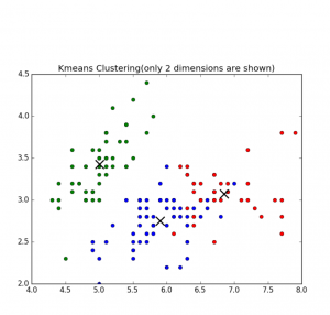
k-means clustering Iris dataset

Fig 1. K-means clustering of Iris dataset
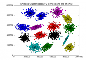

Fig 2. K-means clustering of S1 dataset

Affinity Propagation – performs affinity propagation clustering of data. In statistics and data mining, affinity propagation (AP) is a clustering algorithm based on the concept of “message passing” between data points. Unlike clustering algorithms such as k-means or k-medoids, affinity propagation does not require the number of clusters to be determined or estimated before running the algorithm. Similar to k-medoids, affinity propagation finds “exemplars”, members of the input set that are representative of clusters.[3]

Hierarchical clustering (HC) – (also called hierarchical cluster analysis or HCA) is a method of cluster analysis which seeks to build a hierarchy of clusters. Strategies for hierarchical clustering generally fall into two types:

  • Agglomerative: This is a “bottom up” approach: each observation starts in its own cluster, and pairs of clusters are merged as one moves up the hierarchy.
  • Divisive: This is a “top down” approach: all observations start in one cluster, and splits are performed recursively as one moves down the hierarchy.

In general, the merges and splits are determined in a greedy manner. The results of hierarchical clustering are usually presented in a dendrogram. [4]

Birch algorithm – Back in the 1990s considerable effort has been put into improving the performance of existing algorithms. Among them is BIRCH (Zhang et al., 1996) [5]

BIRCH (balanced iterative reducing and clustering using hierarchies) is an unsupervised data mining algorithm used to perform hierarchical clustering over particularly large data-sets. An advantage of BIRCH is its ability to incrementally and dynamically cluster incoming, multi-dimensional metric data points in an attempt to produce the best quality clustering for a given set of resources (memory and time constraints). In most cases, BIRCH only requires a single scan of the database. [6]

Performance metrics for clustering algorithms

Silhouette refers to a method of interpretation and validation of consistency within clusters of data. The technique provides a succinct graphical representation of how well each object lies within its cluster. It was first described by Peter J. Rousseeuw in 1986.

The silhouette value is a measure of how similar an object is to its own cluster (cohesion) compared to other clusters (separation). The silhouette ranges from -1 to 1, where a high value indicates that the object is well matched to its own cluster and poorly matched to neighboring clusters. If most objects have a high value, then the clustering configuration is appropriate. If many points have a low or negative value, then the clustering configuration may have too many or too few clusters.
The silhouette can be calculated with any distance metric, such as the Euclidean distance or the Manhattan distance.[7]

Here is the python source code how to calculate the silhouette value for k-means clustering


from sklearn import cluster
from sklearn import metrics
import numpy as np


k=2
data = np.array([[1, 2],
              [5, 8],
              [1.5, 1.8],
              [8, 8],
              [1, 0.6],
              [9, 11]])


kmeans = cluster.KMeans(n_clusters=k)
kmeans.fit(data)


labels = kmeans.labels_
centroids = kmeans.cluster_centers_

print ("Cluster id labels for inputted data")
print (labels)
print ("Centroids data")
print (centroids)

print ("\nScore (Opposite of the value of X on the K-means objective which is Sum of distances of samples to their closest cluster center):")
print (kmeans.score(data))

silhouette_score = metrics.silhouette_score(data, labels, metric='euclidean')

print ("Silhouette_score: ")
print (silhouette_score)

Score (Opposite of the value of X on the K-means objective which is Sum of distances of samples to their closest cluster center) – Sum of distances of samples to their closest cluster center.

Large distances corresponds to a big variety in data samples and if the number of data samples is significantly higher than the number of clusters. On the contrary, if all data samples were the same, you would always get a zero distance regardless of number of clusters. [8]

Cophenetic correlation – In statistics, and especially in biostatistics, cophenetic correlation (more precisely, the cophenetic correlation coefficient) is a measure of how faithfully a dendrogram preserves the pairwise distances between the original unmodeled data points. Although it has been most widely applied in the field of biostatistics (typically to assess cluster-based models of DNA sequences, or other taxonomic models), it can also be used in other fields of inquiry where raw data tend to occur in clumps, or clusters. This coefficient has also been proposed for use as a test for nested clusters.[9]

Datasets
The following two datasets will be used:
The Iris flower data set or Fisher’s Iris data set is a multivariate data set – well know data set with N = 150 and k=3 [10] The data set consists of 50 samples from each of three species of Iris (Iris setosa, Iris virginica and Iris versicolor) [10]

S1 – Synthetic 2-d data with N=5000 vectors and k=15 Gaussian cluster [11]

Experiments
Using ML Sandbox tool and above clustering algorithms and datasets the clustering was performed. Screenshots of results of clustering from the tool were collected and presented here (Fig 1-6, Fig 1,2 are shown above)
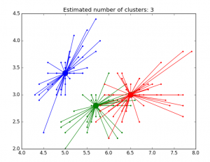

Fig 3. AP clustering of Iris dataset


Fig 4. AP clustering results of Iris dataset
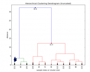

Fig 5. HC Clustering Iris dataset
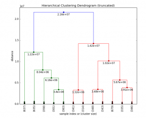

Fig 6. HC clustering S1 dataset

Below in the summary of the above clustering experiments.

Kmeans (sklearn.cluster) AP (sklearn.cluster) HC (scipy.cluster) Birch (sklearn.cluster)
Score (Opposite of Sum of distances of samples to their closest cluster center) Silhouette_score Silhouette_score Cophenetic Correlation Coefficient: Silhouette_score
Iris dataset, 150, D4 -78.85 0.55 0.52 0.87 0.50
S1 dataset, 5000, D2 -8.92e+12 0.71 * 0.69 0.71

*AP did not work well on S1 dataset (but worked well on iris dataset) however there are some other optional parameters that can be used to resolve this. Probably need to be adjust preference parameter. Currently the tool does not allow change it.

From documentation [12] Preference is parameter that can be array-like, shape (n_samples,) or float, and is optional. Preferences for each point – points with larger values of preferences are more likely to be chosen as exemplars. The number of exemplars, ie of clusters, is influenced by the input preferences value. If the preferences are not passed as arguments, they will be set to the median of the input similarities.

ML Sandbox
The above tool was used for clustering data. You need just select algorithm, enter your data and click run. Below are detailed instructions for clustering.
How to use the ML Sandbox
1. Open URL: ML Sandbox
2. Select Clustering method
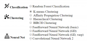
3. Enter data (you can use default small dataset or copy and paste your dataset or dataset from other sites like iris, S1 see links in the references section)
4. Click Run Now
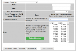
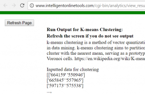
5. Click View Run Results
6. If you do not see results, click refresh button at top left corner. Depending on data set and algorithm you might need wait for a minute or two and click refresh.
Conclusion
We looked at different clustering methods, metrics performance and visualization of clustering results for different datasets. All of this can be done within online tool ML Sandbox Feel free to play with this tool and your data to explore your datasets. Also feel free to provide any feedback or suggestions.

References
1. Hierarchical Clustering: A Simple Explanation
2. k-means clustering
3. Affinity_propagation
4. Hierarchical clustering
5. Cluster_analysis
6. BIRCH
7. Silhouette (clustering)
8. understanding-score-returned-by-scikit-learn-kmeans
9. Cophenetic correlation
10. Iris flower data set
11. Clustering benchmark datasets
12 AffinityPropagation


Extracting Google AdSense and Google Analytics Data for Website Analytics

Recently I decided to get information that is showing for each page of my website Google Analytics account number and all Google AdSense links on this page. Connecting this information with Google Publisher Pages data would be very useful for better analysis and understanding of ads performance.

So I created python script that is doing the following:

1. Opens file with some initial links. The initial links then are extracted into the list in computer memory.
2. Takes first link and extracts HTML text from this link.
3. Extracts Google Analytics account number from HTML. The acconneunt number usually appears on web page code on the line, formatted like this : ‘_uacct = “UA-xxxxxxxxxx”;’ The script extracts UA- number using regular expression.
4. Extracts Google AdSense information from HTML text. AdSense information is displayed within /* */ like below:

google_ad_client = “pub-xxxxxxxxx”;
/* 300×15, created 1/20/17 */
google_ad_slot = “xxxxxxxx”;
Here ‘300×15, created 1/20/17’ is default ad name.

5. Extracts all links from the same HTML text.
6. Adds links to list. Links are added to list only if they are from specific website domain.
7. Outputs extracted information to csv file. The saved information contains url, GA account number and AdSense ad names that are on the page.
8. Repeats steps 2 – 6 while there are links to process.

Here are few examples how the script can be used:

  • Lookup of page for the given ad. For example AdSense is showing clicked link and we want to know what page it was.
  • Check if all pages have GA and AdSense code inserted.
  • Check the count of AdSense ads on the page.
  • Use the data with Google Analytics and AdSense for analysis of revenue variation or conversion rate by ad size for different group of web pages.

Below you can find script source code and flow chart.


# -*- coding: utf-8 -*-

import urllib.request
import lxml.html
import csv
import time
import os
import re
import string
import requests

path="C:\\Users\\Owner\\Desktop\\2017"

filename = path + "\\" + "urlsB.csv" 

filename_info_extracted= path + "\\" + "urls_info_extracted.csv"

urls_to_skip =['search3.cgi']

def load_file(fn):
         start=0
         file_urls=[]       
         with open(fn, encoding="utf8" ) as f:
            csv_f = csv.reader(f)
            for i, row in enumerate(csv_f):
               if i >=  start  :
                 file_urls.append (row)
         return file_urls

def save_extracted_url (fn, row):
    
         if (os.path.isfile(fn)):
             m="a"
         else:
             m="w"
    
       
         with open(fn, m, encoding="utf8", newline='' ) as csvfile: 
             fieldnames = ['url', 'GA', 'GS']
             writer = csv.DictWriter(csvfile, fieldnames=fieldnames)
             if (m=="w"):
                 writer.writeheader()
             writer.writerow(row)


links_processed = []

urlsA= load_file (filename)
print ("Starting navigate...")

url_ind=0 
done=False
while not done:
 u=urlsA[url_ind] 
 new_row={} 
 print (u[0])
 print (u)
 
 try:
  connection = urllib.request.urlopen(u[0])
  print (u[0])
  print ("connected")
  dom =  lxml.html.fromstring(connection.read())
  time.sleep( 12 )
  r = requests.get(u[0])

  # Get the text of the contents
  html_content = r.text
 
  
  pat = re.compile(r"(/\*(.+?)\*/)+", re.MULTILINE)
  if pat.search(html_content) != None:
                         
             str=""
             for match in pat.finditer(html_content):
                   print ("%s: %s" % (match.start(), match.group(1)))
                   str=str+","+ match.group(1)
             new_row['GS'] = str
             
  pat1 = re.compile(r"_uacct(.+?)google_ad_client", re.MULTILINE)
  pat1 = re.compile(r"_uacct(.+?)\"(.+?)\"", re.MULTILINE)
  if pat1.search(html_content) != None:
             
             m=pat1.search(html_content)
             new_row['GA'] = m.group(2)
             
            
  links_processed.append (u) 

  new_row['url'] = u[0]  
  save_extracted_url (filename_info_extracted, new_row)
  url_ind=url_ind+1
   
  
  print (html_content)
  
  links=[]
  for link in dom.xpath('//a/@href'):
      
     a=link.split("?") 
     if "lwebzem" in a[0]:
                
         try:
            links.append (link)
            ind=string.find(link, "?")
            
            if ind >=0:
                 print ( link[:ind])
            else :
                 print (link)
                 
         except :
             print ("EXCP" + link)
         
         skip = False   
         if [link] in links_processed:
               print ("SKIPPED " + link)
               skip=True
         if link in urlsA:
               skip = True
         if urls_to_skip[0] in link:
               skip=True
         if not skip:    
              urlsA.append ([link])
              
         
 except:
     url_ind=url_ind+1        
 if url_ind > len(urlsA) :
     done=True   


Converting Categorical Text Variable into Binary Variables

Sometimes we might need convert categorical feature into multiple binary features. Such situation emerged while I was implementing decision tree with independent categorical variable using python sklearn.tree for the post Building Decision Trees in Python – Handling Categorical Data and it turned out that a text independent variable is not supported.

One of solution would be binary encoding, also called one-hot-encoding when we might code [‘red’,’green’,’blue’] with 3 columns, one for each category, having 1 when the category match and 0 otherwise. [1]

Here we implement the python code that makes such binary encoding. The script looks at text data column and add numerical columns with values 0 or 1 to the original data. If category word exists in the column then it will be 1 in the column for this category, otherwise 0.

The list of categories is initialized in the beginning of the script. Additionally we initialize data source file, number of column with text data, and number of first empty column on right side. The script will add columns on right side starting from first empty column.

The next step in the script is to navigate through each row and do binary conversion and update data.

Below is some example of added binary columns to data input .

Below is full source code.


# -*- coding: utf-8 -*-

import pandas as pd

words = ["adwords", "adsense","mortgage","money","loan"]
data = pd.read_csv('adwords_data5.csv', sep= ',' , header = 0)


total_rows = len(data.index)


y_text_column_index=7
y_column_index=16


for index, w in enumerate(words):
  data[w] = 0   
  col_index=data.columns.get_loc(w)
  
  for x in range (total_rows):
      if w in data.iloc[x,y_text_column_index] :
           data.iloc[x,y_column_index+index]=1
      else :
           data.iloc[x,y_column_index+index]=0  


print (data)

References
1. strings as features in decision tree/random forest
2. Building Decision Trees in Python
3. Building Decision Trees in Python – Handling Categorical Data


Building Decision Trees in Python – Handling Categorical Data

In the post Building Decision Trees in Python we looked at the decision tree with numerical continuous dependent variable. This type of decision trees can be called also regression tree.

But what if we need to use categorical dependent variable? It is still possible to create decision tree and in this post we will look how to create decision tree if dependent variable is categorical data. In this case the decision tree is called classification tree. Classification trees, as the name implies are used to separate the dataset into classes belonging to the response variable. [4] Classification is a typical problem that can be found in such fields as machine learning, predictive analytics, data mining.

Getting Data
For simplicity we will use the same dataset as before but will convert numerical target variable into categorical variable as we want build python code for decision tree with categorical dependent variable.
To convert dependent variable into categorical we use the following simple rule:
if CPC < 22 then CPC = "Low"
else CPC = “High”

For independent variables we will use “keyword” and “number of words” fields.
Keyword (usually it is several words) is a categorical variable. In general it is not the problem as in either case (regression or classification tree), the predictors or independent variables may be categorical or numeric. It is the target variable that determines the type of decision tree needed.[4]

However sklearn.tree (at least the version that is used here) does not support categorical independent variable. See discussion and suggestions on stack overflow [5]. To use independent categorical variable, we will code the categorical feature into multiple binary features. For example, we might code [‘red’,’green’,’blue’] with 3 columns, one for each category, having 1 when the category match and 0 otherwise. This is called one-hot-encoding, binary encoding, one-of-k-encoding or whatever. [5]

Below are shown few rows from the table data. We added 2 columns for categories “insurance”, “Adsense”. We actually have more categories and therefore we added more columns but this is not shown in the table.

For small dataset such conversion can be done manually. But we also created python script in the post Converting Categorical Text Variable into Binary Variables for this specific task. [10]

Keyword Number of words Insurance Adsense CTR Cost Cost (categorical)
car insurance premium 3 1 0 0.012 20 Low
AdSense data 2 0 1 0.025 1061 High

Building the Code
Now we need to build the code. The call for decision tree is looking like this:

clf_gini = DecisionTreeClassifier(criterion = “gini”, random_state = 100,
max_depth=8, min_samples_leaf=4)

we use here criterion Gini index for splitting data.
In the call to export_graphviz we specify class names:

export_graphviz(tree, out_file=f, feature_names=feature_names, filled=True, rounded=True, class_names=[“Low”, “High”] )

The rest of the code is the same as in previous post for regression tree.

Here is the python computer code:


# -*- coding: utf-8 -*-


import pandas as pd
from sklearn.cross_validation import train_test_split
from sklearn.tree import DecisionTreeClassifier
import subprocess

from sklearn.tree import  export_graphviz


def visualize_tree(tree, feature_names):
    
    with open("dt.dot", 'w') as f:
        
        export_graphviz(tree, out_file=f, feature_names=feature_names,  filled=True, rounded=True, class_names=["Low", "High"] )

    command = ["C:\\Program Files (x86)\\Graphviz2.38\\bin\\dot.exe", "-Tpng", "C:\\Users\\Owner\\Desktop\\A\\Python_2016_A\\dt.dot", "-o", "dt.png"]
    
       
    try:
        subprocess.check_call(command)
    except:
        exit("Could not run dot, ie graphviz, to "
             "produce visualization")
    
data = pd.read_csv('adwords_data.csv', sep= ',' , header = 1)


X = data.values[:, [3,17,18,19,20,21,22]]
Y = data.values[:,8]

                           
X_train, X_test, y_train, y_test = train_test_split( X, Y, test_size = 0.3, random_state = 100)                           
                           
clf_gini = DecisionTreeClassifier(criterion = "gini", random_state = 100, 
                               max_depth=8, min_samples_leaf=4)
clf_gini.fit(X_train, y_train)   


visualize_tree(clf_gini, ["Words in Key Phrase", "AdSense",	"Mortgage",	"Money",	"loan", 	"lawyer", 	"attorney"])


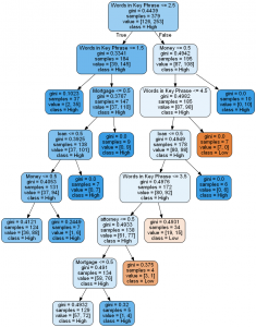
Decision Tree (partial view)

References
1. Decision tree Wikipedia
2. MLlib – Decision Trees
3. Visual analysis of AdWords data: a primer
4. 2 main differences between classification and regression trees
5. strings as features in decision tree/random forest
6. Decision Trees with scikit-learn
7. Classification: Basic Concepts, Decision Trees, and Model Evaluation
8. Understanding decision tree output from export_graphviz
9. Building Decision Trees in Python
10. Converting Categorical Text Variable into Binary Variables


Building Decision Trees in Python

A decision tree is a decision support tool that uses a tree-like graph or model of decisions and their possible consequences, including chance event outcomes, resource costs, and utility. It is one way to display an algorithm.
Decision trees are commonly used in operations research, specifically in decision analysis, to help identify a strategy most likely to reach a goal, but are also a popular tool in machine learning. [1]

Decision trees are widely used since they are easy to interpret, handle categorical features, extend to the multiclass classification setting, do not require feature scaling, and are able to capture non-linearities and feature interactions. [2] Decision trees are also one of the most widely used predictive analytics techniques.

Recently I decided to build python code for decision tree for AdWords data. This was motivated by the post [3] about visual analytics used for AdWords dataset. Below are the main components that I used for implementing decision tree.

Dataset
AdWords dataset – the dataset was obtained on Internet. Below is the table with few rows to show data. Only the columns that were used for decision tree, are shown in the table.

Keyword Number of words CPC Clicks CTR Cost Impressions
car insurance premium 3 176 7 0.012 1399 484
AdSense data 2 119 13 0.025 1061 466

The following independent variables were selected:
Number of words in keyword phrase – this column was added based on the keyword phrase column.
CTR – click through rate

For the dependent variable it was selected CPC – Average Cost per Click.

Python Module
As the dependent variable is numeric and continuos, the regression decision tree from python module sklearn.tree was used in the script:
from sklearn.tree import DecisionTreeRegressor

In sklearn.tree Decision Trees (DTs) are a non-parametric supervised learning method used for classification and regression. The goal is to create a model that predicts the value of a target variable by learning simple decision rules inferred from the data features. [5]

Visualization
For visualization of decision tree graphviz was installed. “Graphviz is open source graph visualization software. Graph visualization is a way of representing structural information as diagrams of abstract graphs and networks. It has important applications in networking, bioinformatics, software engineering, database and web design, machine learning, and in visual interfaces for other technical domains.”

Python Script
The created code consisted of the following steps:
reading data from csv data file
selecting needed columns
splitting dataset for testing and training
initializing DecisionTreeRegressor
visualizing decision tree via function. Note that the path to Graphviz are specified inside of scripts.

Decision tree and Python code are shown below. Online resources used for this post are provided in the reference section.

Decision Tree
Decision Tree

Python computer code:


# -*- coding: utf-8 -*-

import pandas as pd
from sklearn.cross_validation import train_test_split
from sklearn.tree import DecisionTreeRegressor


import subprocess

from sklearn.tree import  export_graphviz


def visualize_tree(tree, feature_names):
    
    with open("dt.dot", 'w') as f:
        
        export_graphviz(tree, out_file=f, feature_names=feature_names,  filled=True, rounded=True )

    command = ["C:\\Program Files (x86)\\Graphviz2.38\\bin\\dot.exe", "-Tpng", "C:\\Users\\Owner\\Desktop\\A\\Python_2016_A\\dt.dot", "-o", "dt.png"]
    
        
    try:
        subprocess.check_call(command)
    except:
        exit("Could not run dot, ie graphviz, to "
             "produce visualization")
    
data = pd.read_csv('adwords_data.csv', sep= ',' , header = 1)


X = data.values[:, [3,13]]
Y = data.values[:,11]

                       
X_train, X_test, y_train, y_test = train_test_split( X, Y, test_size = 0.3, random_state = 100)                           
                           
clf = DecisionTreeRegressor( random_state = 100,
                               max_depth=3, min_samples_leaf=4)
clf.fit(X_train, y_train)   


visualize_tree(clf, ["Words in Key Phrase", "CTR"])

References
1. Decision tree Wikipedia
2. MLlib – Decision Trees
3. Visual analysis of AdWords data: a primer
4. Decision trees in python with scikit_learn and pandas
5. Decision Tree
6. Graphviz – Graph Visualization Software