Machine Learning Stock Prediction with LSTM and Keras – Python Source Code

Python Source Code for Machine Learning Stock Prediction with LSTM and Keras – Python Source Code with LSTM and Keras Below is the code for machine learning stock prediction with LSTM neural network.

# -*- coding: utf-8 -*-

import numpy as np
import pandas as pd
from sklearn import preprocessing
import matplotlib.pyplot as plt


fname="C:\\Users\\stock_data.csv"
data_csv = pd.read_csv (fname)

#how many data we will use 
# (should not be more than dataset length )
data_to_use= 100

# number of training data
# should be less than data_to_use
train_end =70


total_data=len(data_csv)

#most recent data is in the end 
#so need offset
start=total_data - data_to_use


#currently doing prediction only for 1 step ahead
steps_to_predict =1

 
yt = data_csv.iloc [start:total_data ,4]    #Close price
yt1 = data_csv.iloc [start:total_data ,1]   #Open
yt2 = data_csv.iloc [start:total_data ,2]   #High
yt3 = data_csv.iloc [start:total_data ,3]   #Low
vt = data_csv.iloc [start:total_data ,6]    # volume


print ("yt head :")
print (yt.head())

yt_ = yt.shift (-1)
    
data = pd.concat ([yt, yt_, vt, yt1, yt2, yt3], axis =1)
data. columns = ['yt', 'yt_', 'vt', 'yt1', 'yt2', 'yt3']
    
data = data.dropna()
    
print (data)
    
# target variable - closed price
# after shifting
y = data ['yt_']

       
#       closed,  volume,   open,  high,   low    
cols =['yt',    'vt',  'yt1', 'yt2', 'yt3']
x = data [cols]


scaler_x = preprocessing.MinMaxScaler ( feature_range =( -1, 1))
x = np. array (x).reshape ((len( x) ,len(cols)))
x = scaler_x.fit_transform (x)

   
scaler_y = preprocessing. MinMaxScaler ( feature_range =( -1, 1))
y = np.array (y).reshape ((len( y), 1))
y = scaler_y.fit_transform (y)

    
x_train = x [0: train_end,]
x_test = x[ train_end +1:len(x),]    
y_train = y [0: train_end] 
y_test = y[ train_end +1:len(y)]  
x_train = x_train.reshape (x_train. shape + (1,)) 
x_test = x_test.reshape (x_test. shape + (1,))


from keras.models import Sequential
from keras.layers.core import Dense
from keras.layers.recurrent import LSTM
from keras.layers import  Dropout


seed =2016 
np.random.seed (seed)
fit1 = Sequential ()
fit1.add (LSTM (  1000 , activation = 'tanh', inner_activation = 'hard_sigmoid' , input_shape =(len(cols), 1) ))
fit1.add(Dropout(0.2))
fit1.add (Dense (output_dim =1, activation = 'linear'))

fit1.compile (loss ="mean_squared_error" , optimizer = "adam")   
fit1.fit (x_train, y_train, batch_size =16, nb_epoch =25, shuffle = False)

print (fit1.summary())

score_train = fit1.evaluate (x_train, y_train, batch_size =1)
score_test = fit1.evaluate (x_test, y_test, batch_size =1)
print (" in train MSE = ", round( score_train ,4)) 
print (" in test MSE = ", score_test )

   
pred1 = fit1.predict (x_test) 
pred1 = scaler_y.inverse_transform (np. array (pred1). reshape ((len( pred1), 1)))


prediction_data = pred1[-1]     
   

fit1.summary()
print ("Inputs: {}".format(fit1.input_shape))
print ("Outputs: {}".format(fit1.output_shape))
print ("Actual input: {}".format(x_test.shape))
print ("Actual output: {}".format(y_test.shape))
  

print ("prediction data:")
print (prediction_data)


print ("actual data")
x_test = scaler_x.inverse_transform (np. array (x_test). reshape ((len( x_test), len(cols))))
print (x_test)


plt.plot(pred1, label="predictions")


y_test = scaler_y.inverse_transform (np. array (y_test). reshape ((len( y_test), 1)))
plt.plot( [row[0] for row in y_test], label="actual")

plt.legend(loc='upper center', bbox_to_anchor=(0.5, -0.05),
          fancybox=True, shadow=True, ncol=2)

import matplotlib.ticker as mtick
fmt = '$%.0f'
tick = mtick.FormatStrFormatter(fmt)

ax = plt.axes()
ax.yaxis.set_major_formatter(tick)


plt.show()

References
1. Machine Learning Stock Prediction with LSTM and Keras – Python Source Code with LSTM and Keras


Machine Learning Stock Prediction with LSTM and Keras

In this post I will share experiments on machine learning stock prediction with LSTM and Keras with one step ahead. I tried to do first multiple steps ahead with few techniques described in the papers on the web. But I discovered that I need fully understand and test the simplest model – prediction for one step ahead. So I put here the example of prediction of stock price data time series for one next step.

Preparing Data for Neural Network Prediction

Our first task is feed the data into LSTM. Our data is stock price data time series that were downloaded from the web.
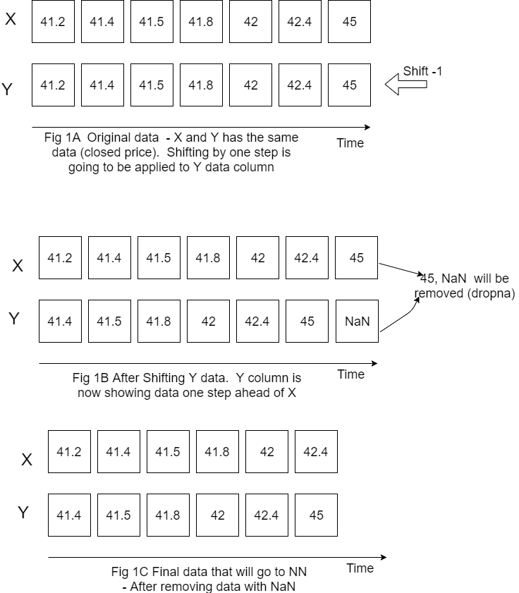
Our interest is closed price for the next day so target variable will be closed price but shifted to left (back) by one step.

Figure below is showing how do we prepare X, Y data.
Please note that I put X Y horizontally for convenience but still calling X, Y as columns.
Also on this figure only one variable (closed price) is showed for X but in the code it is actually more than one variable (it is closed price, open price, volume and high price).

LSTM data input
LSTM data input

Now we have the data that we can feed for LSTM neural network prediction. Before doing this we need also do the following things:

1. Decide how many data we want to use. For example if we have data for 10 years but want use only last 200 rows of data we would need specify start point because the most recent data will be in the end.

#how many data we will use 
# (should not be more than dataset length )
data_to_use= 100

# number of training data
# should be less than data_to_use
train_end =70


total_data=len(data_csv)

#most recent data is in the end 
#so need offset
start=total_data - data_to_use

2. Rescale (normalize) data as below. Here feature_range is tuple (min, max), default=(0, 1) is desired range of transformed data. [1]

scaler_x = preprocessing.MinMaxScaler ( feature_range =( -1, 1))
x = np. array (x).reshape ((len( x) ,len(cols)))
x = scaler_x.fit_transform (x)


scaler_y = preprocessing. MinMaxScaler ( feature_range =( -1, 1))
y = np.array (y).reshape ((len( y), 1))
y = scaler_y.fit_transform (y)

3. Divide data into training and testing set.

x_train = x [0: train_end,]
x_test = x[ train_end +1:len(x),]    
y_train = y [0: train_end] 
y_test = y[ train_end +1:len(y)]  

Building and Running LSTM

Now we need to define our LSTM neural network layers , parameters and run neural network to see how it works.

fit1 = Sequential ()
fit1.add (LSTM (  1000 , activation = 'tanh', inner_activation = 'hard_sigmoid' , input_shape =(len(cols), 1) ))
fit1.add(Dropout(0.2))
fit1.add (Dense (output_dim =1, activation = 'linear'))

fit1.compile (loss ="mean_squared_error" , optimizer = "adam")   
fit1.fit (x_train, y_train, batch_size =16, nb_epoch =25, shuffle = False)

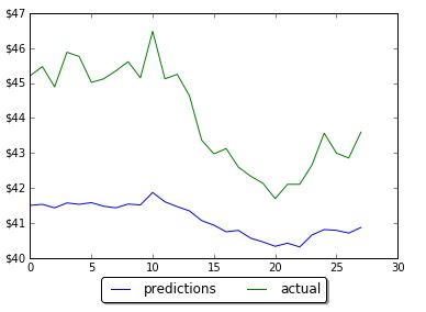
The first run was not good – prediction was way below actual.

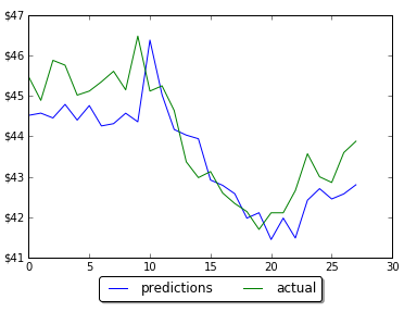
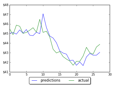
However by changing the number of neurons in LSTM neural network prediction code, it was possible to improve MSE and get predictions much closer to actual data. Below are screenshots of plots of prediction and actual data for LSTM with 5, 60 and 1000 neurons. Note that the plot is showing only testing data. Training data is not shown on the plots. Also you can find below the data for MSE and number of neurons. As the number neorons in LSTM layer is changing there were 2 minimums (one around 100 neurons and another around 1000 neurons)

Results of prediction on LSTM with 5 neurons
Forecasting one step ahead LSTM 60
Results of prediction on LSTM with 60 neurons
Forecasting one step ahead
Results of prediction on LSTM with 1000 neurons

LSTM 5
in train MSE = 0.0475
in test MSE = 0.2714831660102521

LSTM 60
in train MSE = 0.0127
in test MSE = 0.02227417068206705

LSTM 100
in train MSE = 0.0126
in test MSE = 0.018672733913263073

LSTM 200
in train MSE = 0.0133
in test MSE = 0.020082660237026824

LSTM 900
in train MSE = 0.0103
in test MSE = 0.015546535929778267

LSTM 1000
in train MSE = 0.0104
in test MSE = 0.015037054958075455

LSTM 1100
in train MSE = 0.0113
in test MSE = 0.016363980411369994

Conclusion

The final LSTM was running with testing MSE 0.015 and accuracy 97%. This was obtained by changing number of neurons in LSTM. This example will serve as baseline for further possible improvements on machine learning stock prediction with LSTM. If you have any tips or anything else to add, please leave a comment the comment box. The full source code for LSTM neural network prediction can be found here

References
1. sklearn.preprocessing.MinMaxScaler
2. Keras documentation – RNN Layers
3. How to Reshape Input Data for Long Short-Term Memory Networks in Keras
4. Keras FAQ: Frequently Asked Keras Questions
5. Time Series Prediction with LSTM Recurrent Neural Networks in Python with Keras
6.Deep Time Series Forecasting with Python: An Intuitive Introduction to Deep Learning for Applied Time Series Modeling
7. Machine Learning Stock Prediction with LSTM and Keras – Python Source Code


Prediction Data Stock Prices with Prophet

In the previous post I showed how to use the Prophet for time series analysis with python. I used Prophet for data stock price prediction. But it was used only for one stock and only for next 10 days.

In this post we will select more data and will test how accurate can be prediction data stock prices with Prophet.

We will select 5 stocks and will do prediction stock prices based on their historical data. You will get chance to look at the report how error is distributed across different stocks or number of days in forecast. The summary report will show that we can easy get accuracy as high as 96.8% for stock price prediction with Prophet for 20 days forecast.

Data and Parameters

The five stocks that we will select are the stocks in the price range between $20 – $50. The daily historical data are taken from the web.

For time horizon we will use 20 days. That means that we will save last 20 prices for testing and will not use for forecasting.

Experiment

For this experiment we use python script with the main loop that is iterating for each stock. Inside of the loop, Prophet is doing forecast and then error is calculated and saved for each day in forecast:

   model = Prophet() #instantiate Prophet
   model.fit(data);
   future_stock_data = model.make_future_dataframe(periods=steps_ahead, freq = 'd')
   forecast_data = model.predict(future_stock_data)

   step_count=0
   # save actual data 
   for index, row in data_test.iterrows():
    
     results[ind][step_count][0] = row['y']
     results[ind][step_count][4] = row['ds']
     step_count=step_count + 1
   
   # save predicted data and calculate error
   count_index = 0   
   for index, row in forecast_data.iterrows():
     if count_index >= len(data)  :
       
        step_count= count_index - len(data)
        results[ind][step_count][1] = row['yhat']
        results[ind][step_count][2] = results[ind][step_count][0] -  results[ind][step_count][1]
        results[ind][step_count][3] = 100 * results[ind][step_count][2] / results[ind][step_count][0]
      
     count_index=count_index + 1

Later on (as shown in the above python source code) we count error as difference between actual closed price and predicted. Also error is calculated in % for each day for each stock using the formula:

Error(%) = 100*(Actual-Predicted)/Actual

Results
The detailed result report can be found here. In this report you can see how error is distributed across different days. You can note that there is no significant increase in error with 20 days of forecast and the error always has the same sign for all 20 days.

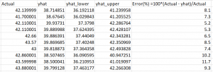
Below is the summary of error and accuracy for our selected 5 stocks. Also added the column the year of starting point of data range that was used for forecast. It turn out that all 5 stocks have different historical data range. The shortest data range was starting in the middle of 2016.

prediction data stock prices with Prophet summary results
prediction data stock prices with Prophet summary of results

Overall results for accuracy are not great. Only one stock got good accuracy 96.8%.
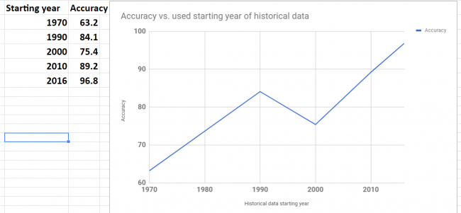
Accuracy was varying for different stocks. To investigate variation I plot graph of accuracy and beginning year of historical data. The plot is shown below. Looks like there is a correlation between data range used for forecast and accuracy. This makes sense – as the data in the further past may be do more harm than good.

Looking at the plot below we see that the shortest historical range (just about for one year) showed the best accuracy.

prediction data stock prices with Prophet - accuracy vs used data range
prediction data stock prices with Prophet – accuracy vs used data range

Conclusion
We did not get good results (except one stock) in our experiments but we got the knowledge about possible range and distribution of error over the different stocks and time horizon (up to 20 days). Also it looks promising to try do forecast with different historical data range to check how it will affect performance. It would be interesting to see if the best accuracy that we got for one stock can be achieved for other stocks too.

I hope you enjoyed this post about using Prophet for prediction data stock prices. If you have any tips or anything else to add, please leave a comment in the reply box below.

Here is the script for stock data forecasting with python using Prophet.

import pandas as pd
from fbprophet import Prophet

steps_ahead = 20
fname_path="C:\\Users\\stock data folder"

fnames=['fn1.csv','fn2.csv', 'fn3.csv', 'fn4.csv', 'fn5.csv']
# output fields: actual, predicted, error, error in %, date
fields_number = 6

results= [[[0 for i in range(len(fnames))] for j in range(steps_ahead)] for k in range(fields_number)]

for ind in range(5):
 
   fname=fname_path + "\\" + fnames[ind]
  
   data = pd.read_csv (fname)

   #keep only date and close
   #delete Open, High,	Low  , Adj CLose, Volume
   data.drop(data.columns[[1, 2, 3,5,6]], axis=1)
   data.columns = ['ds', 'y', "", "", "", "", ""]
  
   data_test = data[-steps_ahead:]
   print (data_test)
   data = data[:-steps_ahead]
   print (data)
     
   model = Prophet() #instantiate Prophet
   model.fit(data);
   future_stock_data = model.make_future_dataframe(periods=steps_ahead, freq = 'd')
   forecast_data = model.predict(future_stock_data)
   print (forecast_data[['ds', 'yhat', 'yhat_lower', 'yhat_upper']].tail(12))

   step_count=0
   for index, row in data_test.iterrows():
    
     results[ind][step_count][0] = row['y']
     results[ind][step_count][4] = row['ds']
     step_count=step_count + 1
   
  
   count_index = 0   
   for index, row in forecast_data.iterrows():
     if count_index >= len(data)  :
       
        step_count= count_index - len(data)
        results[ind][step_count][1] = row['yhat']
        results[ind][step_count][2] = results[ind][step_count][0] -  results[ind][step_count][1]
        results[ind][step_count][3] = 100 * results[ind][step_count][2] / results[ind][step_count][0]
      
     count_index=count_index + 1

for z in range (5):        
  for i in range (steps_ahead):
    temp=""
    for j in range (5):
          temp=temp + " " + str(results[z][i][j])
    print (temp)
   
   
  print (z)  


Time Series Analysis with Python and Prophet

Recently Facebook released Prophet – open source software tool for forecasting time series data.
Facebook team have implemented in Prophet two trend models that can cover many applications: a saturating growth model, and a piecewise linear model. [4]

With growth model Prophet can be used for prediction growth/decay – for example for modeling growth of population or website traffic. By default, Prophet uses a linear model for its forecast.

In this post we review main features of Prophet and will test it on prediction of stock data prices for next 10 business days. We will use python for time series programming with Prophet.

How to Use Prophet for Time Series Analysis with Python

Here is the minimal python source code to create forecast with Prophet.

import pandas as pd
from fbprophet import Prophet

The input columns should have headers as ‘ds’ and ‘y’. In the code below we run forecast for 180 days ahead for stock data, ds is our date stamp data column, and y is actual time series column

fname="C:\\Users\\data analysis\\gm.csv"
data = pd.read_csv (fname)

data.columns = ['ds', 'y']
model = Prophet() 
model.fit(data); #fit the model
future_stock_data = model.make_future_dataframe(periods=180, freq = 'd')
forecast_data = model.predict(future_stock_data)
print ("Forecast data")
model.plot(forecast_data)

The result of the above code will be graph shown below.

time series analysis python using Prophet

Time series model consists of three main model components: trend, seasonality, and holidays.
We can print components using the following line

model.plot_components(forecast_data)
time series analysis python - components
time series analysis python – components

Can Prophet be Used for Data Stock Price Prediction?

It is interesting to know if Prophet can be use for financial market price forecasting. The practical question is how accurate forecasting with Prophet for stock data prices? Data analytics for stock market is known as hard problem as many different events influence stock prices every day. To check how it works I made forecast for 10 days ahead using actual stock data and then compared Prophet forecast with actual data.

The error was calculated for each day for data stock price (closed price) and is shown below

Data stock price prediction analysis

Based on obtained results the average error is 7.9% ( this is 92% accuracy). In other words the accuracy is sort of low for stock prices prediction. But note that all errors have the same sign. May be Prophet can be used better for prediction stock market direction? This was already mentioned in another blog [2].
And also looks like the error is not changing much with the the time horizon, at least within first 10 steps. Forecasts for days 3,4,5 even have smaller error than for the day 1 and 2.

Further looking at more data would be interesting and will follow soon. Bellow is the full python source code.


import pandas as pd
from fbprophet import Prophet


fname="C:\\Users\\GM.csv"
data = pd.read_csv (fname)
data.columns = ['ds', 'y']
model = Prophet() #instantiate Prophet
model.fit(data); #fit the model with your dataframe

future_stock_data = model.make_future_dataframe(periods=10, freq = 'd')
forecast_data = model.predict(future_stock_data)

print ("Forecast data")
print (forecast_data[['ds', 'yhat', 'yhat_lower', 'yhat_upper']].tail(12))
	
model.plot(forecast_data)
model.plot_components(forecast_data)

References
1. Stock market forecasting with prophet
2. Can we predict stock prices with Prophet?
3. Saturating Forecasts
4. Forecasting at Scale


Regression and Classification Decision Trees – Building with Python and Running Online

According to survey [1] Decision Trees constitute one of the 10 most popular data mining algorithms.
Decision trees used in data mining are of two main types:
Classification tree analysis is when the predicted outcome is the class to which the data belongs.
Regression tree analysis is when the predicted outcome can be considered a real number (e.g. the price of a house, or a patient’s length of stay in a hospital).[2]

In the previous posts I already covered how to create Regression Decision Trees with python:

Building Decision Trees in Python
Building Decision Trees in Python – Handling Categorical Data

In this post you will find more simplified python code for classification and regression decision trees. Online link to run decision tree also will be provided. This is very useful if you want see results immediately without coding.

To run the code provided here you need just change file path to file containing data. The Decision Trees in this post are tested on simple artificial dataset that was motivated by doing feature selection for blog data:

Getting Data-Driven Insights from Blog Data Analysis with Feature Selection

Dataset
Our dataset consists of 3 columns in csv file and shown below. It has 2 independent variables (features or X columns) – categorical and numerical, and dependent numerical variable (target or Y column). The script is assuming that the target column is the last column. Below is the dataset that is used in this post:


X1	X2	Y
red	1	100
red	2	99
red	1	85
red	2	100
red	1	79
red	2	100
red	1	100
red	1	85
red	2	100
red	1	79
blue	2	22
blue	1	20
blue	2	21
blue	1	13
blue	2	10
blue	1	22
blue	2	20
blue	1	21
blue	2	13
blue	1	10
blue	1	22
blue	2	20
blue	1	21
blue	2	13
blue	1	10
blue	2	22
blue	1	20
blue	2	21
blue	1	13
green	2	10
green	1	22
green	2	20
green	1	21
green	2	13
green	1	10
green	2	22
green	1	20
green	1	13
green	2	22
green	1	20
green	2	21
green	1	13
green	2	10

You can use dataset with different number of columns for independent variables without changing the code.

For converting categorical variable to numerical we use here pd.get_dummies(dataframe) method from pandas library. Here dataframe is our input data. So the column with “green”, “red”, “yellow” will be transformed in 3 columns with 0,1 values in each (one hot encoding scheme). Below are the few first rows after converting:


N   X2  X1_blue  X1_green  X1_red    Y
0    1      0.0       0.0     1.0  100
1    2      0.0       0.0     1.0   99
2    1      0.0       0.0     1.0   85
3    2      0.0       0.0     1.0  100

Python Code
Two scripts are provided here – regressor and classifier. For classifier the target variable should be categorical. We use however same dataset but convert numerical continuous variable to classes with labels (A,B,C) within the script based on inputted bin ranges ([15,50,100] which means bins 0-15, 15.001-50, 50.001-100). We use this after applying get_dummies

What if you have categorical target? Calling get_dummies will convert it to numerical too but we do not want this. In this case you need specify explicitly what columns need to be converted via parameter columns As per the documentation:
columns : list-like, default None. This is column names in the DataFrame to be encoded. If columns is None then all the columns with object or category dtype will be converted. [3]
In our example we would need to do specify column X1 like this:
dataframe=pd.get_dummies(dataframe, columns=[“X1”])

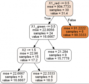
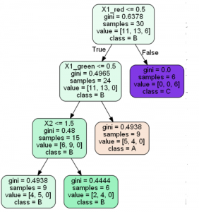
The results of running scripts are decision trees shown below:
Decision Tree Regression
Decision Tree Classification
Running Decision Trees Online
In case you do not want to play with python code, you can run Decision Tree algorithms online at ML Sandbox
All that you need is just enter data into the data fields, here are the instructions:

  1. Go to ML Sandbox
  2. Select Decision Classifier OR Decision Regressor
  3. Enter data (first row should have headers) OR click “Load Default Values” to load the example data from this post. See screenshot below
  4. Click “Run Now“.
  5. Click “View Run Results
  6. If you do not see yet data wait for a minute or so and click “Refresh Page” and you will see results
  7. Note: your dependent variable (target variable or Y variable) should be in most right column. Also do not use space in the words (header and data)

    Conclusion
    Decision Trees belong to the top 10 machine learning or data mining algorithms and in this post we looked how to build Decision Trees with python. The source code provided is the end of this post. We looked also how do this if one or more columns are categorical. The source code was tested on simple categorical and numerical example and provided in this post. Alternatively you can run same algorithm online at ML Sandbox

    References

    1. Top 10 Machine Learning Algorithms for Beginners
    2. Decision Tree Learning
    3. pandas.get_dummies

    Here is the python computer code of the scripts.
    DecisionTreeRegressor

    
    # -*- coding: utf-8 -*python computer code-
    
    import pandas as pd
    from sklearn.cross_validation import train_test_split
    from sklearn.tree import DecisionTreeRegressor
    
    
    import subprocess
    
    from sklearn.tree import  export_graphviz
    
    
    def visualize_tree(tree, feature_names):
        
        with open("dt.dot", 'w') as f:
            
            export_graphviz(tree, out_file=f, feature_names=feature_names,  filled=True, rounded=True )
    
        command = ["C:\\Program Files (x86)\\Graphviz2.38\\bin\\dot.exe", "-Tpng", "C:\\Users\\Owner\\Desktop\\A\\Python_2016_A\\dt.dot", "-o", "dt.png"]
        
            
        try:
            subprocess.check_call(command)
        except:
            exit("Could not run dot, ie graphviz, to "
                 "produce visualization")


    filename = "C:\\Users\\Owner\\Desktop\\A\\Blog Analytics\\data1.csv"
    dataframe = pd.read_csv(filename, sep= ',' )


    cols = dataframe.columns.tolist()
    last_col_header = cols[-1]
    
    
    dataframe=pd.get_dummies(dataframe)
    cols = dataframe.columns.tolist()
    
    cols.insert(len(dataframe.columns)-1, cols.pop(cols.index(last_col_header)))
    dataframe = dataframe.reindex(columns= cols)
    
    print (dataframe)


    array = dataframe.values
    X = array[:,0:len(dataframe.columns)-1]  
    Y = array[:,len(dataframe.columns)-1]   
    print ("--X----")
    print (X)
    print ("--Y----")
    print (Y)
    
                           
    X_train, X_test, y_train, y_test = train_test_split( X, Y, test_size = 0.3, random_state = 100)                           
                               
    clf = DecisionTreeRegressor( random_state = 100,
                                   max_depth=3, min_samples_leaf=4)
    clf.fit(X_train, y_train)   
    
    visualize_tree(clf, dataframe.columns)
    

    DecisionTreeClassifier

    
    # -*- coding: utf-8 -*-
    
    import pandas as pd
    from sklearn.cross_validation import train_test_split
    from sklearn.tree import DecisionTreeClassifier
    
    import subprocess
    
    from sklearn.tree import  export_graphviz
    
    
    def visualize_tree(tree, feature_names, class_names):
        
        with open("dt.dot", 'w') as f:
            
            export_graphviz(tree, out_file=f, feature_names=feature_names,  filled=True, rounded=True, class_names=class_names )
    
        command = ["C:\\Program Files (x86)\\Graphviz2.38\\bin\\dot.exe", "-Tpng", "C:\\Users\\Owner\\Desktop\\A\\Python_2016_A\\dt.dot", "-o", "dt.png"]
        
            
        try:
            subprocess.check_call(command)
        except:
            exit("Could not run dot, ie graphviz, to "
                 "produce visualization")


    values=[15,50,100]
    def convert_to_label (a):
        count=0
        for v in values:
            if (a <= v) :
                return chr(ord('A') + count)
            else:
                count=count+1
        
        
    filename = "C:\\Users\\Owner\\Desktop\\A\\Blog Analytics\\data1.csv"
    dataframe = pd.read_csv(filename, sep= ',' )
    
    cols = dataframe.columns.tolist()
    last_col_header = cols[-1]
    dataframe=pd.get_dummies(dataframe)
    cols = dataframe.columns.tolist()
    
    
    print (dataframe)
    
    
    for index, row in dataframe.iterrows():
           dataframe.loc[index, "Y"] = convert_to_label(dataframe.loc[index, "Y"])


    cols.insert(len(dataframe.columns)-1, cols.pop(cols.index('Y')))
    dataframe = dataframe.reindex(columns= cols)
    
    print (dataframe)
    
    array = dataframe.values
    X = array[:,0:len(dataframe.columns)-1]  
    Y = array[:,len(dataframe.columns)-1]   
    print ("--X----")
    print (X)
    print ("--Y----")
    print (Y)
                           
    X_train, X_test, y_train, y_test = train_test_split( X, Y, test_size = 0.3, random_state = 100)                           
                               
    
    clf = DecisionTreeClassifier(criterion = "gini", random_state = 100,
                                   max_depth=3, min_samples_leaf=4)
    
    
    clf.fit(X_train, y_train)   
    
    clm=dataframe[last_col_header]
    clmvalues = clm.unique()
    visualize_tree(clf, dataframe.columns, clmvalues )