Machine Learning Stock Prediction with LSTM and Keras

In this post I will share experiments on machine learning stock prediction with LSTM and Keras with one step ahead. I tried to do first multiple steps ahead with few techniques described in the papers on the web. But I discovered that I need fully understand and test the simplest model – prediction for one step ahead. So I put here the example of prediction of stock price data time series for one next step.

Preparing Data for Neural Network Prediction

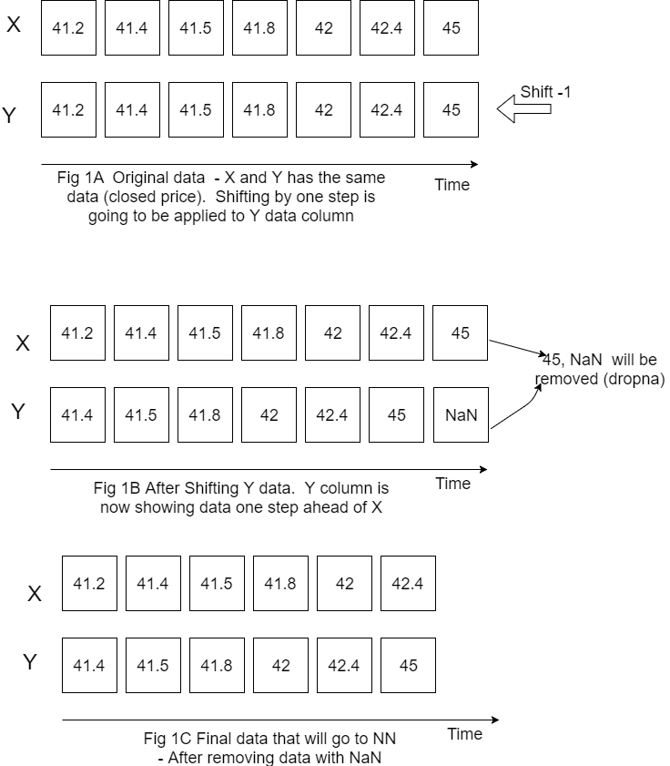
Our first task is feed the data into LSTM. Our data is stock price data time series that were downloaded from the web.
Our interest is closed price for the next day so target variable will be closed price but shifted to left (back) by one step.

Figure below is showing how do we prepare X, Y data.
Please note that I put X Y horizontally for convenience but still calling X, Y as columns.
Also on this figure only one variable (closed price) is showed for X but in the code it is actually more than one variable (it is closed price, open price, volume and high price).

LSTM data input
LSTM data input

Now we have the data that we can feed for LSTM neural network prediction. Before doing this we need also do the following things:

1. Decide how many data we want to use. For example if we have data for 10 years but want use only last 200 rows of data we would need specify start point because the most recent data will be in the end.

#how many data we will use 
# (should not be more than dataset length )
data_to_use= 100

# number of training data
# should be less than data_to_use
train_end =70


total_data=len(data_csv)

#most recent data is in the end 
#so need offset
start=total_data - data_to_use

2. Rescale (normalize) data as below. Here feature_range is tuple (min, max), default=(0, 1) is desired range of transformed data. [1]

scaler_x = preprocessing.MinMaxScaler ( feature_range =( -1, 1))
x = np. array (x).reshape ((len( x) ,len(cols)))
x = scaler_x.fit_transform (x)


scaler_y = preprocessing. MinMaxScaler ( feature_range =( -1, 1))
y = np.array (y).reshape ((len( y), 1))
y = scaler_y.fit_transform (y)

3. Divide data into training and testing set.

x_train = x [0: train_end,]
x_test = x[ train_end +1:len(x),]    
y_train = y [0: train_end] 
y_test = y[ train_end +1:len(y)]  

Building and Running LSTM

Now we need to define our LSTM neural network layers , parameters and run neural network to see how it works.

fit1 = Sequential ()
fit1.add (LSTM (  1000 , activation = 'tanh', inner_activation = 'hard_sigmoid' , input_shape =(len(cols), 1) ))
fit1.add(Dropout(0.2))
fit1.add (Dense (output_dim =1, activation = 'linear'))

fit1.compile (loss ="mean_squared_error" , optimizer = "adam")   
fit1.fit (x_train, y_train, batch_size =16, nb_epoch =25, shuffle = False)

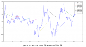
The first run was not good – prediction was way below actual.

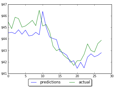
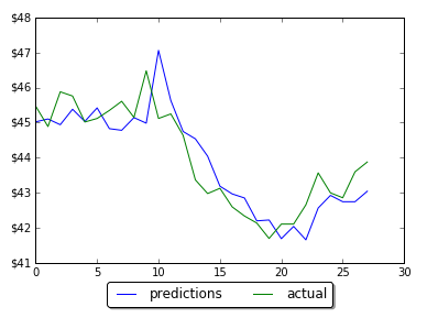
However by changing the number of neurons in LSTM neural network prediction code, it was possible to improve MSE and get predictions much closer to actual data. Below are screenshots of plots of prediction and actual data for LSTM with 5, 60 and 1000 neurons. Note that the plot is showing only testing data. Training data is not shown on the plots. Also you can find below the data for MSE and number of neurons. As the number neorons in LSTM layer is changing there were 2 minimums (one around 100 neurons and another around 1000 neurons)
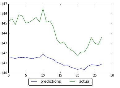
Results of prediction on LSTM with 5 neurons
Forecasting one step ahead LSTM 60
Results of prediction on LSTM with 60 neurons
Forecasting one step ahead
Results of prediction on LSTM with 1000 neurons

LSTM 5
in train MSE = 0.0475
in test MSE = 0.2714831660102521

LSTM 60
in train MSE = 0.0127
in test MSE = 0.02227417068206705

LSTM 100
in train MSE = 0.0126
in test MSE = 0.018672733913263073

LSTM 200
in train MSE = 0.0133
in test MSE = 0.020082660237026824

LSTM 900
in train MSE = 0.0103
in test MSE = 0.015546535929778267

LSTM 1000
in train MSE = 0.0104
in test MSE = 0.015037054958075455

LSTM 1100
in train MSE = 0.0113
in test MSE = 0.016363980411369994

Conclusion

The final LSTM was running with testing MSE 0.015 and accuracy 97%. This was obtained by changing number of neurons in LSTM. This example will serve as baseline for further possible improvements on machine learning stock prediction with LSTM. If you have any tips or anything else to add, please leave a comment the comment box. The full source code for LSTM neural network prediction can be found here

References
1. sklearn.preprocessing.MinMaxScaler
2. Keras documentation – RNN Layers
3. How to Reshape Input Data for Long Short-Term Memory Networks in Keras
4. Keras FAQ: Frequently Asked Keras Questions
5. Time Series Prediction with LSTM Recurrent Neural Networks in Python with Keras
6.Deep Time Series Forecasting with Python: An Intuitive Introduction to Deep Learning for Applied Time Series Modeling
7. Machine Learning Stock Prediction with LSTM and Keras – Python Source Code


Prediction Data Stock Prices with Prophet

In the previous post I showed how to use the Prophet for time series analysis with python. I used Prophet for data stock price prediction. But it was used only for one stock and only for next 10 days.

In this post we will select more data and will test how accurate can be prediction data stock prices with Prophet.

We will select 5 stocks and will do prediction stock prices based on their historical data. You will get chance to look at the report how error is distributed across different stocks or number of days in forecast. The summary report will show that we can easy get accuracy as high as 96.8% for stock price prediction with Prophet for 20 days forecast.

Data and Parameters

The five stocks that we will select are the stocks in the price range between $20 – $50. The daily historical data are taken from the web.

For time horizon we will use 20 days. That means that we will save last 20 prices for testing and will not use for forecasting.

Experiment

For this experiment we use python script with the main loop that is iterating for each stock. Inside of the loop, Prophet is doing forecast and then error is calculated and saved for each day in forecast:

   model = Prophet() #instantiate Prophet
   model.fit(data);
   future_stock_data = model.make_future_dataframe(periods=steps_ahead, freq = 'd')
   forecast_data = model.predict(future_stock_data)

   step_count=0
   # save actual data 
   for index, row in data_test.iterrows():
    
     results[ind][step_count][0] = row['y']
     results[ind][step_count][4] = row['ds']
     step_count=step_count + 1
   
   # save predicted data and calculate error
   count_index = 0   
   for index, row in forecast_data.iterrows():
     if count_index >= len(data)  :
       
        step_count= count_index - len(data)
        results[ind][step_count][1] = row['yhat']
        results[ind][step_count][2] = results[ind][step_count][0] -  results[ind][step_count][1]
        results[ind][step_count][3] = 100 * results[ind][step_count][2] / results[ind][step_count][0]
      
     count_index=count_index + 1

Later on (as shown in the above python source code) we count error as difference between actual closed price and predicted. Also error is calculated in % for each day for each stock using the formula:

Error(%) = 100*(Actual-Predicted)/Actual

Results
The detailed result report can be found here. In this report you can see how error is distributed across different days. You can note that there is no significant increase in error with 20 days of forecast and the error always has the same sign for all 20 days.

Below is the summary of error and accuracy for our selected 5 stocks. Also added the column the year of starting point of data range that was used for forecast. It turn out that all 5 stocks have different historical data range. The shortest data range was starting in the middle of 2016.

prediction data stock prices with Prophet summary results
prediction data stock prices with Prophet summary of results

Overall results for accuracy are not great. Only one stock got good accuracy 96.8%.
Accuracy was varying for different stocks. To investigate variation I plot graph of accuracy and beginning year of historical data. The plot is shown below. Looks like there is a correlation between data range used for forecast and accuracy. This makes sense – as the data in the further past may be do more harm than good.

Looking at the plot below we see that the shortest historical range (just about for one year) showed the best accuracy.

prediction data stock prices with Prophet - accuracy vs used data range
prediction data stock prices with Prophet – accuracy vs used data range

Conclusion
We did not get good results (except one stock) in our experiments but we got the knowledge about possible range and distribution of error over the different stocks and time horizon (up to 20 days). Also it looks promising to try do forecast with different historical data range to check how it will affect performance. It would be interesting to see if the best accuracy that we got for one stock can be achieved for other stocks too.

I hope you enjoyed this post about using Prophet for prediction data stock prices. If you have any tips or anything else to add, please leave a comment in the reply box below.

Here is the script for stock data forecasting with python using Prophet.

import pandas as pd
from fbprophet import Prophet

steps_ahead = 20
fname_path="C:\\Users\\stock data folder"

fnames=['fn1.csv','fn2.csv', 'fn3.csv', 'fn4.csv', 'fn5.csv']
# output fields: actual, predicted, error, error in %, date
fields_number = 6

results= [[[0 for i in range(len(fnames))] for j in range(steps_ahead)] for k in range(fields_number)]

for ind in range(5):
 
   fname=fname_path + "\\" + fnames[ind]
  
   data = pd.read_csv (fname)

   #keep only date and close
   #delete Open, High,	Low  , Adj CLose, Volume
   data.drop(data.columns[[1, 2, 3,5,6]], axis=1)
   data.columns = ['ds', 'y', "", "", "", "", ""]
  
   data_test = data[-steps_ahead:]
   print (data_test)
   data = data[:-steps_ahead]
   print (data)
     
   model = Prophet() #instantiate Prophet
   model.fit(data);
   future_stock_data = model.make_future_dataframe(periods=steps_ahead, freq = 'd')
   forecast_data = model.predict(future_stock_data)
   print (forecast_data[['ds', 'yhat', 'yhat_lower', 'yhat_upper']].tail(12))

   step_count=0
   for index, row in data_test.iterrows():
    
     results[ind][step_count][0] = row['y']
     results[ind][step_count][4] = row['ds']
     step_count=step_count + 1
   
  
   count_index = 0   
   for index, row in forecast_data.iterrows():
     if count_index >= len(data)  :
       
        step_count= count_index - len(data)
        results[ind][step_count][1] = row['yhat']
        results[ind][step_count][2] = results[ind][step_count][0] -  results[ind][step_count][1]
        results[ind][step_count][3] = 100 * results[ind][step_count][2] / results[ind][step_count][0]
      
     count_index=count_index + 1

for z in range (5):        
  for i in range (steps_ahead):
    temp=""
    for j in range (5):
          temp=temp + " " + str(results[z][i][j])
    print (temp)
   
   
  print (z)  


Time Series Analysis with Python and Prophet

Recently Facebook released Prophet – open source software tool for forecasting time series data.
Facebook team have implemented in Prophet two trend models that can cover many applications: a saturating growth model, and a piecewise linear model. [4]

With growth model Prophet can be used for prediction growth/decay – for example for modeling growth of population or website traffic. By default, Prophet uses a linear model for its forecast.

In this post we review main features of Prophet and will test it on prediction of stock data prices for next 10 business days. We will use python for time series programming with Prophet.

How to Use Prophet for Time Series Analysis with Python

Here is the minimal python source code to create forecast with Prophet.

import pandas as pd
from fbprophet import Prophet

The input columns should have headers as ‘ds’ and ‘y’. In the code below we run forecast for 180 days ahead for stock data, ds is our date stamp data column, and y is actual time series column

fname="C:\\Users\\data analysis\\gm.csv"
data = pd.read_csv (fname)

data.columns = ['ds', 'y']
model = Prophet() 
model.fit(data); #fit the model
future_stock_data = model.make_future_dataframe(periods=180, freq = 'd')
forecast_data = model.predict(future_stock_data)
print ("Forecast data")
model.plot(forecast_data)

The result of the above code will be graph shown below.

time series analysis python using Prophet

Time series model consists of three main model components: trend, seasonality, and holidays.
We can print components using the following line

model.plot_components(forecast_data)
time series analysis python - components
time series analysis python – components

Can Prophet be Used for Data Stock Price Prediction?

It is interesting to know if Prophet can be use for financial market price forecasting. The practical question is how accurate forecasting with Prophet for stock data prices? Data analytics for stock market is known as hard problem as many different events influence stock prices every day. To check how it works I made forecast for 10 days ahead using actual stock data and then compared Prophet forecast with actual data.

The error was calculated for each day for data stock price (closed price) and is shown below

Data stock price prediction analysis

Based on obtained results the average error is 7.9% ( this is 92% accuracy). In other words the accuracy is sort of low for stock prices prediction. But note that all errors have the same sign. May be Prophet can be used better for prediction stock market direction? This was already mentioned in another blog [2].
And also looks like the error is not changing much with the the time horizon, at least within first 10 steps. Forecasts for days 3,4,5 even have smaller error than for the day 1 and 2.

Further looking at more data would be interesting and will follow soon. Bellow is the full python source code.


import pandas as pd
from fbprophet import Prophet


fname="C:\\Users\\GM.csv"
data = pd.read_csv (fname)
data.columns = ['ds', 'y']
model = Prophet() #instantiate Prophet
model.fit(data); #fit the model with your dataframe

future_stock_data = model.make_future_dataframe(periods=10, freq = 'd')
forecast_data = model.predict(future_stock_data)

print ("Forecast data")
print (forecast_data[['ds', 'yhat', 'yhat_lower', 'yhat_upper']].tail(12))
	
model.plot(forecast_data)
model.plot_components(forecast_data)

References
1. Stock market forecasting with prophet
2. Can we predict stock prices with Prophet?
3. Saturating Forecasts
4. Forecasting at Scale


10 New Top Resources on Machine Learning from Around the Web

For this post I put new and most interesting machine learning resources that I recently found on the web. This is the list of useful resources in such areas like stock market forecasting, text mining, deep learning, neural networks and getting data from Twitter. Hope you enjoy the reading.

1. Stock market forecasting with prophet – this post belongs to series of posts about using Prophet which is the tool for producing high quality forecasts for time series data that has multiple seasonality with linear or non-linear growth. You will find here different techniques for stock data forecasting.
Prophet is open source software released by Facebook’s Core Data Science team. It is available for download on CRAN and PyPI.

2. Python For Finance: Algorithmic Trading – Another post about stock data analysis with python. This tutorial introduces you to algorithmic trading, and much more.

3. Recommendation and trend analysis is interesting topic. You can read this post to find out how to improve algorithms: recommendation-engine-for-trending-products-in-python In this post author is proposing new trending products algorithm in order to increase serendipity. This will allow to show to user something the user would not expect, but still could find interesting.

4. Word2Vec word embedding tutorial in Python and TensorFlow This tutorial is covering “Word2Vec” technique. This methodology is used in NLP to efficiently convert words into numeric vectors.

5. Best Practices for Document Classification with Deep Learning In this post you will find review of some best practices how to use deep learning for text classification. From the examples in this post you will discover different type of Convolutional Neural Networks (CNN) architecture.

6. How to Develop a Deep Learning Bag-of-Words Model for Predicting Movie Review Sentiment In this post you will find how to use deep learning model for sentiment analysis. The model is simple feedforward network with fully connected layers.

7. How to Clean Text for Machine Learning with Python – Here you will find great and complete tutorial for text preprocessing with python. Also links to resources for further learning are provided too.

8. Gathering Tweets with Python. This tutorial guides you in setting up a system for collecting Tweets.

9. Twitter Data Mining: A Guide To Big Data Analytics Using Python Here you can also find how to connect to Twitter and extract some tweets.

10. Stream data from Twitter using Python This post will show you how to get all identification information required for connecting to Twitter. Also you will find here how to receive tweets via the stream from Twitter.


Forecasting Time Series Data with Convolutional Neural Networks

Convolutional neural networks(CNN) is increasingly important concept in computer science and finds more and more applications in different fields. Many posts on the web are about applying convolutional neural networks for image classification as CNN is very useful type of neural networks for image classification. But convolutional neural networks can also be used for applications other than images, such as time series prediction. This post is reviewing existing papers and web resources about applying CNN for forecasting time series data. Some resources also contain python source code.

Deep neural networks opened new opportunities for time series prediction. New types of neural networks such as LSTM (variant of the RNN), CNN were applied for time series forecasting. For example here is the link for predicting time series with LSTM. [1] You can find here also the code. The code provides nice graph with ability to compare actual data and predicted data. (See figure below, sourced from [1]) Predictions start at different points of time so you can see and compare performance for several predictions.

Time series with LSTM

Below review is showing different approaches that can be used for forecasting time series data with convolutional neural networks.

1. Raw Data
The simplest way to feed data into neural network is to use raw data. Here is the link [2] to results of experiments with different types of neural networks including CNN. In this study stock data such as Date,Open,High,Low,Close,Volume,Adj Close were used with 3 types of networks: MLP, CNN and RNN.

CNN architecture was used as 2-layer convolutional neural network (combination of convolution and max-pooling layers) with one fully-connected layer. To improve performance the author suggests using different features (not only scaled time series) like some technical indicators, volume of sales.
According to [12] it is common to periodically insert a Pooling layer in-between successive Convolution layers in a CNN architecture. Its function is to progressively reduce the spatial size of the representation to reduce the amount of parameters and computation in the network, and hence to also control overfitting. The Pooling Layer operates independently on every depth slice of the input and resizes it spatially, using the MAX operation.

2. Automatic Selection of Features
Transforming data before inputting to neural network is common practice. We can use feature based methods like described here in Feature-selection-time-series-forecasting-python or filtering methods like removing trend, seasonality or low pass / high pass filtering.
With deep learning it is possible to lean features automatically. For example in one research the authors introduce a deep learning framework for multivariate time series classification: Multi-Channels Deep Convolutional Neural Networks (MCDCNN). Multivariate time series are separated into univariate ones and perform feature learning on each univariate series individually. Then a
normal MLP is concatenated at the end of feature learning to do classification. [3]
The CNN architecture consists of 2 layer CNN (combination of filter, activation and pooling layers) and 2 Fully connected layers that represent classification MLP.

3. Fully Convolutional Neural Network (FCN)
In this study different neural network architectures such as Multilayer Perceptrons, Fully convolutional NN (FCN), Residual Network are proposed. For FCN authors build the final networks by stacking three convolution blocks with the filter sizes {128, 256, 128} in each block. Unlike the MCNN and MC-CNN, any pooling operation is excluded. This strategy helps to prevent overfitting. Batch normalization is applied to speed up the convergence speed and help improve generalization.

After the convolution blocks, the features are fed into a global average pooling layer instead of a fully connected layer, which largely reduces the number of weights. The final label is produced by a softmax layer. [4] Thus the architecture of neural network consists of three convolution blocks and global average pooling and softmax layers in the end.

4. Different Data Transformations
In this study [5] CNNs were trained with different data transformations, which included: the entire dataset, spatial clustering, and PCA decomposition. Data was also fit to the hidden modules of a Clockwork Recurrent Neural Network. This type of recurrent network (CRNN) has the advantage of maintaining a high-temporal-resolution memory in its hidden layers after training.

This network also overcomes the problem of the vanishing gradient found in other RNNs by partitioning the neurons in its hidden layers as different ”sub-clocks” that are able to capture the input to the network at different time steps. Here you can find more about CRNN [11]. According to this paper a clockwork RNN architecture is similar to a simple RNN with an input, output and hidden layer. The hidden layer is partitioned into g modules each with its own clock rate. Within each module the neurons are fully interconnected.

5. Analysing Multiple Time Series Relationships
This paper [6] focuses on analyzing multiple time series relationships such as correlations between them. Authors show that deep learning methods for time series processing are comparable to the other approaches and have wide opportunities for further improvement. Range of methods is discussed and code optimisations is applied for the convolutional neural network for the forecasting time series data domain.

6. Data Augmentation
In this study two approaches are proposed to artificially increase the size of training sets. The first one is based on data-augmentation techniques. The second one consists in mixing different training sets and learning the network in a semi-supervised way. The authors show that these two approaches improve the overall classification performance.

7. Encoding data as image
Another methodology for time series with convolutional neural networks that got popular with deep learning is encoding data as the image. Here data is encoded as images which feed to neural network. This enables the use of techniques from computer vision for classification.
Here [8] is the link where python script can be found for encoding data as image. It encodes data into formats such as GAF, MTF. The script has the dependencies on python modules such as Numpy, Pandas, Matplolib and Cpickle.

Theory of using image encoded data is described in [9]. In this paper a novel framework proposes to encode time series data as different types of images, namely, Gramian Angular Fields (GAF) and Markov Transition Fields (MTF).

Learning Traffic as Images:
This paper [10] proposes a convolutional neural network (CNN)-based method that learns traffic as images and predicts large-scale, network-wide traffic speed with a high accuracy. Spatiotemporal traffic dynamics are converted to images describing the time and space relations of traffic flow via a two-dimensional time-space matrix. A CNN is applied to the image following two consecutive steps: abstract traffic feature extraction and network-wide traffic speed prediction. CNN architecture consists of several convolutional and pooling layers and fully connected layer in the end for prediction.

Conclusion

Deep learning and convolutional neural networks created new opportunities for forecasting time series data domain. The above text presents different techniques that can be used in time series prediction with convolutional neural networks. The common part that we can see in most of studies is that feature extraction can be done via deep learning automatically in CNN or in other words, CNNs can learn features on their own. Below you can see architecture of CNN at very high level. The actual implementations can vary in different ways, some of them were shown above.

CNN Architecture for Forecasting Time Series Data

References

1. LSTM NEURAL NETWORK FOR TIME SERIES PREDICTION
2. Neural networks for algorithmic trading. Part One — Simple time series forecasting
3. Time Series Classification Using Multi-Channels Deep Convolutional Neural Networks
4. Time Series Classification from Scratch with Deep Neural Networks: A Strong Baseline
5. Assessing Neuroplasticity with Convolutional and Recurrent Neural Networks
6. Signal Correlation Prediction Using Convolutional Neural Networks
7. Data Augmentation for Time Series Classification using Convolutional Neural Networks.
8. Imaging-time-series-to-improve-classification-and-imputation
9. Encoding Time Series as Images for Visual Inspection and Classification Using
Tiled Convolutional Neural Networks

10. Learning Traffic as Images: A Deep Convolutional Neural Network for Large-Scale Transportation Network Speed Prediction
11. A Clockwork RNN
12. CS231n Convolutional Neural Networks for Visual Recognition