Reinforcement Learning Example for Planning Tasks Using Q Learning and Dyna-Q

What is Planning Process

Planning is the process of finding a sequence of actions (steps), which if executed by an
agent result in the achievement of a set of predefined goals. The sequence of actions mentioned above is also referred to as plan. Planning is studied within Reinforcement Learning and Automated Planning that are subfields of Machine Learning and Artificial Intelligence. [1]

Planning can be used in production, here [5] you can find reinforcement learning example applied to learn an approximately optimal strategy for controlling the stations of a production line in order to meet the demand. The goal in this thesis was to create schedule for machines such as press and oven, running in production environment.

In our day to day life we do planning without using any knowledge about Reinforcement Learning or Artificial Intelligence. For example when we create plan of actions for completion project or plan of tasks for the week or month. Using Reinforcement Learning for planning we can save time, find better strategies, eliminate human error.

In this post we will look at typical planning problem of finding actions needed to complete some specific tasks. This is very practical problem as it can be used for making our everyday schedule or for achieving our goals.

Combining Q Learning with Dyna

We will investigate how to apply Reinforcement Learning for planning of actions to complete tasks using algorithm Dyna-Q proposed by R. Sutton and based on combining Dyna and Q learning.

Dyna is most common and often used solution to speed up the learning procedure in Reinforcement Learning. [2],[3] In our experiment we will see how it impact on speed.

Under Dyna the action taken is computed rapidly as a function of the situation, but the
mapping implemented by that system is continually adjusted by a planning process and the planner is not restricted to planning about the current situation. [2]

Q-learning is a model free method which means that there is no need to maintain a separate
structure for the value function and the policy but only the Q-value function. The Dyna-Q
architecture is simpler as two data structures have been replaced with one. [1]

We will look at more details of Dyna-Q framework after we define our environment and problem.

Problem Description

As mentioned above we will do planning of actions that are needed to complete tasks. Given some goals and set of actions we are interesting to know what action we need to take now in order to get the best result in the end.

Lets say by the end of week I need complete project in Applied Machine Learning and project in Reinforcement Learning. I have some rewards for completion of each project as 3 and 10. This means that completion of Reinforcement Learning is more important for whatever reason.

Lets assume I need to put specific number of time – 2 and 3 time units to complete end goal for each project. Time unit can be just 1 hour for this example. I am working only in the evening each day and each day I can make only one action. I have only 5 times to pick.

While I need to put only 2 units of time to complete my weekly goal on Machine Learning project, I still can work on this project after putting 2 unit of time, possibly doing something for next week or for extra credit. Reward is calculated only in the end of week.

The diagram of one of possible path would look like this:

Planning Diagram
Planning Diagram

On this diagram the green indicates path that produces the max reward 13 as the agent was able to complete both goals.

Simplification

As this is the first post on reinforcement learning for planning, we pick very simple problem. And even without calculations we can say that the optimal schedule is when we allocate 2 units for ML project and 3 units for another project and our maximum reward can be 13.

Thus in this example we did few simplifications:
the number of actions is the same as the number of goals. This makes easy a little bit programming for now.
The number of time units needed to complete task is not changing. This is not always true. In real situation we often realize that something that we planned, will take longer time or may be not possible at all at the current moment.

Despite of the above simplification, the program still has a lot to learn.
How would it create action plan for completion the given tasks by the end of specific time period?

Solution

The code here is based on dyna-q for maze problem[4]. It has 2 modules for programming environment and Reinforcement Learning algorithm. Additionally it has main module which run loop with episods.

Our solution consists of two parts:
1. Reinforcement Learning Q learning where we use observed value and update the table with state, action, reward. Here we create action.
2. Dyna part – where we do simulations and also update state action reward after each simulation. Basically we choose randomly state and action, define next state and reward and update the table in same way as in 1.

Out table is pandas data frame shown on flowchart on right side.
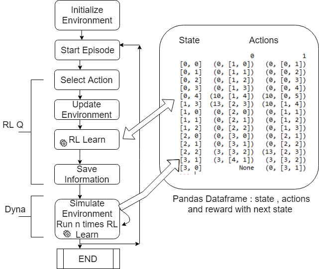
Reinforcement Learning and Planning – Dyna-Q Algorithm

To run this reinforcement learning example you can use python source code from the links below:

Reinforcement Learning Dyna-Q Planning Environment
Reinforcement Learning Dyna-Q
Reinforcement Learning Dyna-Q Run Planning

Results

We run 3 different agents:

1. Random Agent – action is always picked randomly
2. RL Agent – we use only observed values, no simulations are performed. So we use only Q learning.
3. Dyna Q – we use Q learning and Dyna simulations.

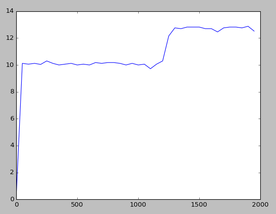
The results are shown on charts below. Here we output average reward for each 50 episods.

Random Agent Run Result
Only RL Q Learning Agent Run Result
RL Dyna-Q Agent Run Result

The random agent was not able to understand that there is better option with reward 13.
RL agent performed better than random, was able to pick reward at 13 however it took long way.
Dyna Q agent was able to pick reward 13 after only 100 episods. The average however about 12.5 So there is some room for improvement.
Still it is not bad considering that we did not do any specific tune up of parameters.

Next Steps

We learned algorithms for reinforcement learning such as Q learning and Dyna-Q techniques that can be used for planning. By adding Dyna part the learning was significantly accelerated.

Next actions would be improve performance, use reinforcement learning deep learning net and make more general environment setup.

References
1. Reinforcement Learning and Automated Planning: A Survey
2. Planning by Incremental Dynamic Programming R. S. Sutton
3. Dyna
4. Reinforcement Learning Methods and Tutorials
5. Reinforcement learning for planning of a simulated production line Gustaf Ehn, Hugo Werner February 27, 2018

Artificial Intelligence – Neural Networks Applications in Seismic Prospecting

TUSHAR website


Global map

Introduction

Large volumes of hydrocarbons remain to be found in the world. Finding and extracting these hydrocarbons is difficult and expensive. We believe that under-utilization of data, and of the existing subsurface knowledge base, are at least partly responsible for the disappointing exploration performance. Furthermore, we argue that the incredibly rich subsurface dataset available can be used much more efficiently to deliver much more precise predictions, and to thus support more profitable investment decisions during hydrocarbon exploration and production.

In this section we will argue that Artificial Intelligence (AI), i.e. Machine Learning-based technology, which leverages algorithms that can learn and make predictions directly from data, represents one way to contribute to exploration and production success. One key advantage of AI is the technology’s ability to efficiently handle very large volumes of multidimensional data, thus saving time and cost and, therefore, allowing human resources to be deployed to other, perhaps more creative tasks. Another advantage is AI or Machine Learning applications is ability to detect complex, multidimensional patterns that are not readily detectable by humans.

We will show in detail how Deep Neural Networks can automate a process in seismic velocity analysis, which usually take days to be done manually. Firstly there will be a brief section describing the process of velocity analysis, then we will move on and integrate the process with Neural Networks and Deep Learning.

Seismic Velocity Analysis

Understanding of the subsurface velocities are very important as they are indicators or various features and also the presence of hydrocarbons or not. With the understanding for the subsurface features we can interpret the traps where hydrocarbon or gases maybe be present.

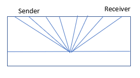
A seismic source and a receiver is kept on a surface. Source produce a wave which penetrates the earth and gets reflected or refracted at several boundaries under the surface and are recorded back by the receiver on the surface. The data that we collect have information of the subsurface structural variations and we then use various methods to interpret them. Seismic Velocity Analysis is a process of getting subsurface velocities at different depths using the data that we just collected.

We will be using Semblance Curves to get the stacking velocities from the Seismic Section. Semblance peaks are picked using Neural Network trained on previously handpicked data.

Semblance Curves

Semblance analysis is a process used in the refinement and study of seismic data. The use of this technique along with other methods makes it possible to greatly increase the resolution of the data despite the presence of background noise. This new data is usually easier to interpret when trying to deduce the underground structure of an area.

Semblance Curve has velocity at its horizontal axis and time at its vertical axis. What our goal is to get a maximum value for each time unit in vertical axis. The values in the curve range from 0 to 1. Theoretically there can be just one maximum value at a time unit but in practice due to noise in our data we get bands with many maximums. It becomes hard to interpret which value is the correct velocity value, so we have to try out each value and see which one flattens our Seismic traces the best. It is a very tedious job to manually pick the value, so here we have trained a neural network which will automatically pick the maximum in each time unit.

Generating Semblance Curves

Semblance Curves were generated using an open source software called Madagascar. The data that we used is also available open source and is the data from Viking Graben Region. You can check the instructions on how to generate Semblance Curves by looking at instructions provided at Madagascar official website. Madagascar comes with an API for attaching the code written in software to any custom build program in many languages. In our case, we will attach this with our tensorflow neural network written in python.

Deep Neural Network

The data that creates the semblance curve is put into numpy array. We have a set of hand picked peaks for our training data set.

We created a simple Multi Layer perceptron with 4 hidden layers and used Adam optimization algorithm to fit the parameters by learning from the hand picked values for our data set. For this we utilized tensorflow functions as below:
optimizer=tf.train.AdamOptimizer(learning_rate=learning_rate).minimize(cost)

The data set has 2400 CMP gathers and 1500 time units in each CMP gather. A gather is a collection of seismic traces that have some common geometric attribute. In our case we use common mid-point (CMP) gather (See Figure below).

The data is huge and it took 15 hours to train and after training the parameters were tested on Nankai dataset (Comes with madagascar software), it gave the output in 10 minutes and achieved an accuracy of 85.67%.

To get python source code, click this link to deep neural network code

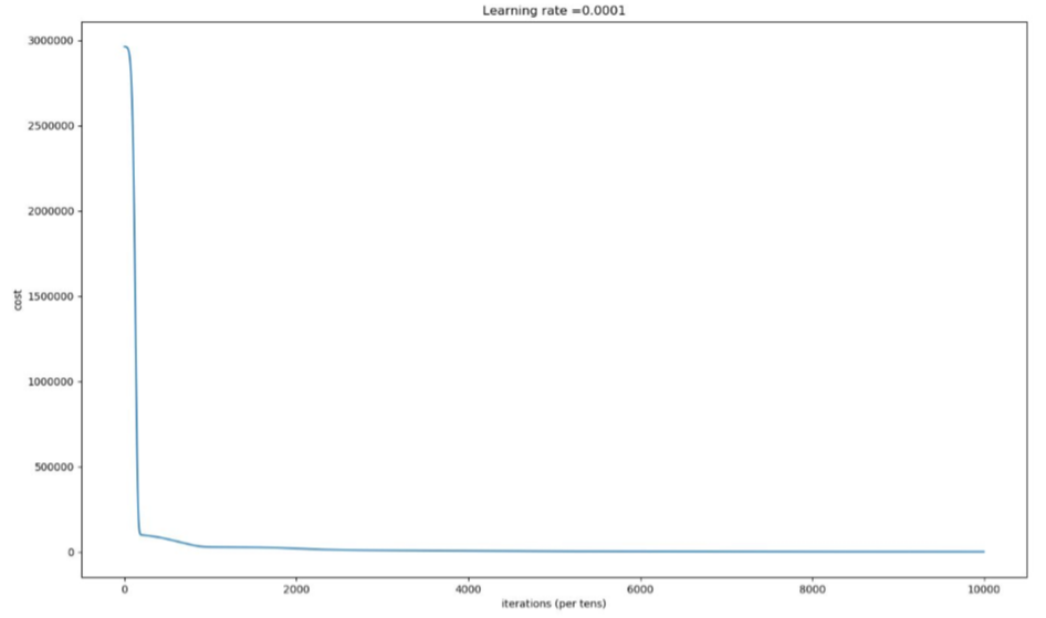
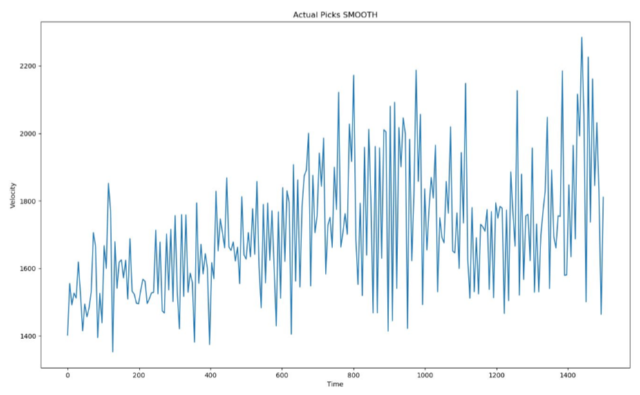
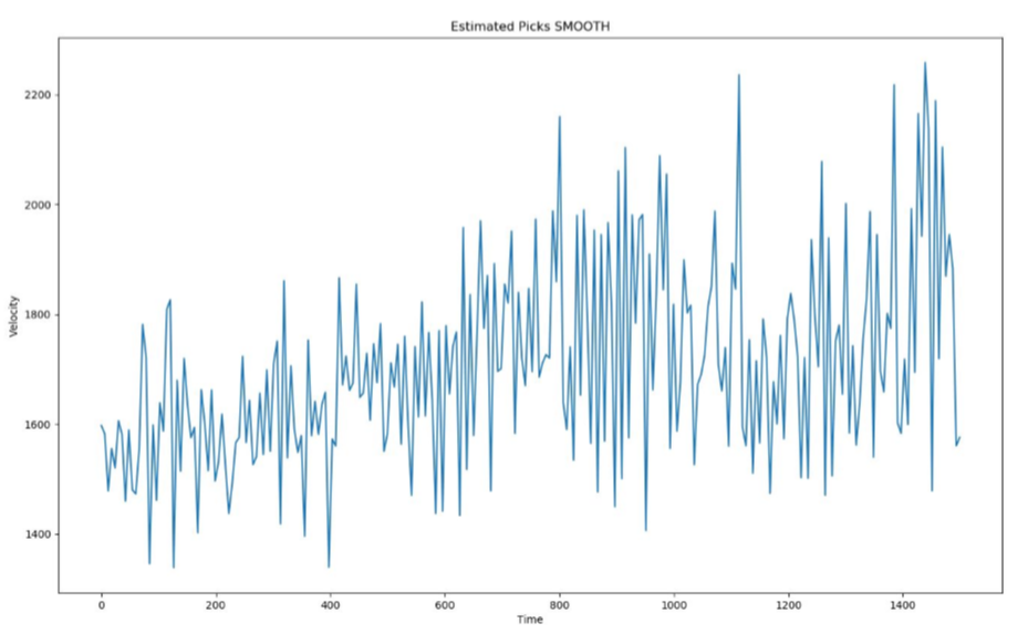
Following are the graphs for Actual Velocities of the region recorded then the velocities estimated by the Neural Network and lastly the learning curve of our neural net.

Conclusion

We can see from the graphs above that Estimated velocities are very close to the actual velocities. Training a neural network takes hours but once trained it reproduces results in minutes. This method saves days of manually picking the peaks which will give us the velocity hence speeding up the process.

References
1. VG Data Madagascar
2. Link to data from Viking Graben Region
3. Gather
4. Neural Networks – Applications Seismic Prospecting Neural Network Code


Everyday Examples of Machine Learning Applications

Artificial Intelligence and Machine Learning applications is one of the most hottest topics in the industry today. Robots, self driving cars, intelligent chatbots and many other innovations are coming to our work and life.
In this post we will look at few machine learning less known applications that were covered in some of previous posts. We will see how machine learning impact our work and life and how we can benefit from this.

Artificial Intelligence – Neural Networks Applications in Seismic Prospecting

Machine learning allows to automate different processes that we use in the work environment. Even if the process is complex like seismic velocity analysis, which usually take days to be done manually. Neural Networks and Deep Learning can be used for speeding up the process and save days of manually picking the peaks.
For more details refer to Neural Networks Applications in Seismic Prospecting post with the example of Multi Layer perceptron.
As result of this saving workers can use their time for more interesting tasks. Thus due to AI and ML the jobs will become more interesting and creative but will require more skills for people.

Correlation Data Analysis Between Food and Mood

food and mood

In the post Machine Learning for Correlation Data Analysis Between Food and Mood machine learning was applied to estimate correlation between eating sweet food and mood state. The moderate correlation (0.4) was detected. Also it was detected some delay (5-6 days) between food intake and change of mood. This corresponds with observation that swing mood may appear in several days, not on the same or next day after eating sweet food.
How we can benefit from this – by controlling food we can control our mood at some degree. One thing is just know that this is bad food that need to be avoided or minimized, another thing to know some numbers – in how many days it will be affected, how strong is the impact? The latest leads to more motivation take actions on food. This helps avoid excuses like “yes, I know it is a bad thing, but may be small quantity is not counted”.

Inferring Causes and Effects from Daily Data

Sample of data after one hot encoding

In the post Inferring Causes and Effects from Daily Data we applied machine learning techniques for learning relationsip bettween data. Here our interest is the date from our actions.

Doing different activities we might be interesting how they impact each other. For example, if we visit different links on Internet, we might want to know how this action impacts our motivation for doing some specific things. In other words we are interesting in inferring importance of causes for effects from our daily activities data.

In this post we will look at few ways to detect relationships between actions and results using machine learning algorithms and python. We create python code to use two machine learning algorithms helped us to estimate the importance of our features (or actions) for our Y variable.

With more data getting collected and available, we will be using more machine learning for making better actions.

Topic modeling

Topic modeling with textacy

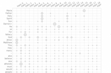
We use topic modeling for discovering topics that occur in a set of documents. Topic modeling applications help us organize collection of text documents (posts, search results, articles), provide quick overview of contents and useful insights. Machine learning has different methods and modules to solve this task. For example, textacy module has a lot of functionality for processing data after applying NLP. This is why python textacy module looks very promising.
And this is also why in the post Topic Modeling Python and Textacy textacy was used for topic modeling. And it showed that it is very easy to do than with other module, for example gensim. This is the trend that we can see – as new module come out we can do more with less.

Conclusion

The above 4 examples of machine learning applications confirm that in the coming years more processes will be automated, some manual labor tasks will be changed to more creative and interesting processes and we will be getting more insights for actions and decisions from our data.

References
1. Topic modeling


Applied Machine Learning Classification for Decision Making

Making the good decision is the challenge that we often have. So, in this post, we will look at how applied machine learning classification can be used for the process of decision making.

The simple and quick approach to make decision is follow our past experience of similar situations. Usually we use compiling a list of pros and cons, asking someone for help or searching on the web. According to [1] we have two systems in our brain: logical and intuitive system:

“With every decision you take, every judgement you make, there is a battle in your mind – a battle between intuition and logic.”

“Most of the beliefs or opinions you have come from an automatic response. But then your logical mind invents a reason why you think or believe something.”

Most of the time our intuitive system is working efficiently, taking charge of all the thousands of decisions we make each day. But our intuitive system can be biased in many ways. For example it can be biased toward the latest unsuccessful outcome.

Besides this our memory can not remember a lot of information so we can not use efficiently all our past information and experience. That’s why people created tools like decision matrix that can help to improve decision making. In the next section we will look at techniques that facilitates using our rational decision making.

Decision Making

Decision Matrix

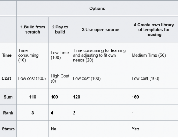
More advanced approach for making decision is score each possible option. In this approach we score each option against some criteria or feature. For example for the candidate product that we need to buy we are looking at price, quality, service and safety features. This approach results in creating decision matrix for analysis of possible options.

Below is an example of decision matrix [3] for choosing strategy for building some software project. Here we score 4 options based on the time to build and cost. The score is on the scale 0 (worst) – 100 (best). After we score each cell for time and cost rows, we can get sum of scores, rank and then make our choice (see last 3 rows)

Decision Matrix Example

There are also other, similar to decision matrix tools: belief decision matrix[3], Pugh Matrix[4].
These tools allow do comparison analysis of available options vs features and this enforces our mind logically evaluate and rank as much as possible pros and cons based on some numerical metrics.

However there are some limitations also. Incorrect selection criteria will obviously lead to the wrong conclusion. Poorly defined criteria can have multiple interpretations. For example too low can mean different things. With many rows or columns it becomes labor intensive to fill out the matrix.

Machine Learning Approach for Making Decision

Machine learning techniques can also help us improve decision making and even solve some of the above limitations. For example with Feature Engineering we can evaluate what criteria are important for decision.

In machine learning making decision can be viewed as assigning or predicting correct label (for example buy, not buy) based on data for the item features. In the field of machine learning or AI this is known as classification problem.

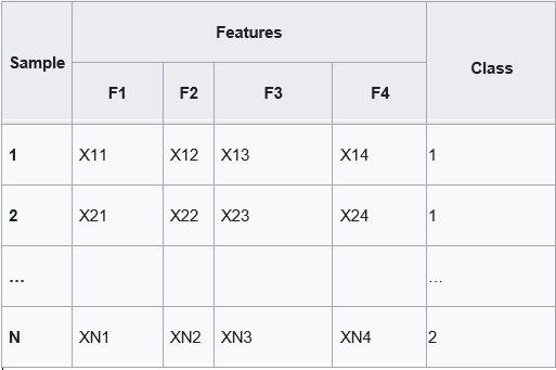
Classification algorithms learn correct decisions from data. Below is the example of training data that we input to machine learning classification algorithm. (Xij represent some numerical values)

Classification problem

Our options (decisions) are now represented by class label (most right column), criteria are represented by features. So we now switched columns with rows. Using training data like above we train classifier and then use it to choose the class (make decision) for new data.

There are different classification algorithms such as decision tree, SVM, Naive Bayes, neural network classification. In this post we will look at classification with neural network.
We will use Keras neural network with 2 dense layers.

Per Keras documentation[5] Dense layer implements the operation:
output = activation(dot(input, kernel) + bias)
where activation is the element-wise activation function passed as the activation argument,
kernel is a weights matrix created by the layer,
and bias is a bias vector created by the layer (only applicable if use_bias is True).

So we can see that the dense layer is performing similar math that we were doing in decision matrix.

Python Source Code for Neural Network Classification Algorithms

Finally, below is the python source code for classification problem. To test this code we will use iris dataset. This dataset has 3 classes and 4 features. Our task here to make the classifier able to assign correct label class.

# -*- coding: utf-8 -*-

from keras.utils import to_categorical
from sklearn import datasets

iris = datasets.load_iris()

# Create feature matrix
X = iris.data
print (X)

# Create target vector
y = iris.target
y = to_categorical(y, num_classes=3)
print (y)

from sklearn.model_selection import train_test_split

x_train, x_test, y_train, y_test = train_test_split( X, y, test_size=0.33, random_state=42)

print (x_train)
print (y_train)

from keras.models import Sequential
from keras.layers import Dense

model = Sequential()
model.add(Dense(32, input_shape=(4,), activation='relu',  name='L1'))
model.add(Dense(3, activation='softmax', name='L2'))
model.compile(optimizer='rmsprop',
              loss='categorical_crossentropy',
              metrics=['accuracy'])

print('Model Summary:')
print(model.summary())

model.fit(x_train, y_train, verbose=2, batch_size=10, epochs=100)
output = model.evaluate(x_test, y_test)

print('Final test loss: {:4f}'.format(output[0]))
print('Final test accuracy: {:4f}'.format(output[1]))


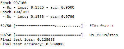
Below are results of neural network run.

Results of neural network run

As we can see our classifier is able to make correct decisions with 98% accuracy.

Thus we investigated different approaches for making decision. We saw how machine learning can be applied to this too. Specifically we looked at neural network classification algorithm for selecting correct label.
I would love to hear what types of decision making tools do you use for making decisions? Also feel free to provide feedback or suggestions.

References
1. How do we really make decisions?
2. What Is a Decision Matrix? Definition and Examples
3. Decision matrix From Wikipedia, the free encyclopedia
4. The Systems Engineering Tool Box
5. Keras Documentation


Inferring Causes and Effects from Daily Data

Doing different activities we often are interesting how they impact each other. For example, if we visit different links on Internet, we might want to know how this action impacts our motivation for doing some specific things. In other words we are interesting in inferring importance of causes for effects from our daily activities data.

In this post we will look at few ways to detect relationships between actions and results using machine learning algorithms and python.

Our data example will be artificial dataset consisting of 2 columns: URL and Y.
URL is our action and we want to know how it impacts on Y. URL can be link0, link1, link2 wich means links visited, and Y can be 0 or 1, 0 means we did not got motivated, and 1 means we got motivated.

The first thing we do hot-encoding link0, link1, link3 in 0,1 and we will get 3 columns as below.

Sample of data after one hot encoding

So we have now 3 features, each for each URL. Here is the code how to do hot-encoding to prepare our data for cause and effect analysis.

filename = "C:\\Users\\drm\\data.csv"
dataframe = pandas.read_csv(filename)

dataframe=pandas.get_dummies(dataframe)
cols = dataframe.columns.tolist()
cols.insert(len(dataframe.columns)-1, cols.pop(cols.index('Y')))
dataframe = dataframe.reindex(columns= cols)

print (len(dataframe.columns))

#output
#4 

Now we can apply feature extraction algorithm. It allows us select features according to the k highest scores.

# feature extraction
test = SelectKBest(score_func=chi2, k="all")
fit = test.fit(X, Y)
# summarize scores
numpy.set_printoptions(precision=3)
print ("scores:")
print(fit.scores_)

for i in range (len(fit.scores_)):
    print ( str(dataframe.columns.values[i]) + "    " + str(fit.scores_[i]))
features = fit.transform(X)

print (list(dataframe))

numpy.set_printoptions(threshold=numpy.inf)


scores:
[11.475  0.142 15.527]
URL_link0    11.475409836065575
URL_link1    0.14227166276346598
URL_link2    15.526957539965377
['URL_link0', 'URL_link1', 'URL_link2', 'Y']


Another algorithm that we can use is <strong>ExtraTreesClassifier</strong> from python machine learning library sklearn.


from sklearn.ensemble import ExtraTreesClassifier
from sklearn.feature_selection import SelectFromModel

clf = ExtraTreesClassifier()
clf = clf.fit(X, Y)
print (clf.feature_importances_)  
model = SelectFromModel(clf, prefit=True)
X_new = model.transform(X)
print (X_new.shape)      

#output
#[0.424 0.041 0.536]
#(150, 2)


The above two machine learning algorithms helped us to estimate the importance of our features (or actions) for our Y variable. In both cases URL_link2 got highest score.

There exist other methods. I would love to hear what methods do you use and for what datasets and/or problems. Also feel free to provide feedback or comments or any questions.

References
1. Feature Selection For Machine Learning in Python
2. sklearn.ensemble.ExtraTreesClassifier

Below is python full source code

# -*- coding: utf-8 -*-
import pandas
import numpy
from sklearn.feature_selection import SelectKBest
from sklearn.feature_selection import chi2


filename = "C:\\Users\\drm\\data.csv"
dataframe = pandas.read_csv(filename)

dataframe=pandas.get_dummies(dataframe)
cols = dataframe.columns.tolist()
cols.insert(len(dataframe.columns)-1, cols.pop(cols.index('Y')))
dataframe = dataframe.reindex(columns= cols)

print (dataframe)
print (len(dataframe.columns))


array = dataframe.values
X = array[:,0:len(dataframe.columns)-1]  
Y = array[:,len(dataframe.columns)-1]   
print ("--X----")
print (X)
print ("--Y----")
print (Y)


# feature extraction
test = SelectKBest(score_func=chi2, k="all")
fit = test.fit(X, Y)
# summarize scores
numpy.set_printoptions(precision=3)
print ("scores:")
print(fit.scores_)

for i in range (len(fit.scores_)):
    print ( str(dataframe.columns.values[i]) + "    " + str(fit.scores_[i]))
features = fit.transform(X)

print (list(dataframe))

numpy.set_printoptions(threshold=numpy.inf)
print ("features")
print(features)


from sklearn.ensemble import ExtraTreesClassifier
from sklearn.feature_selection import SelectFromModel

clf = ExtraTreesClassifier()
clf = clf.fit(X, Y)
print ("feature_importances")
print (clf.feature_importances_)  
model = SelectFromModel(clf, prefit=True)
X_new = model.transform(X)
print (X_new.shape)