Combining Machine Learning and Data Scraping

I often come across web posts about extracting data (data scraping) from websites. For example recently in [1] Scrapy tool was used for web scraping with Python. Once we get scraping data we can use extracted information in many different ways. As computer algorithms evolve and can do more, the number of cases where machine learning is used to get insights from extracted data is increasing. In the case of extracted data from text, exploring commonly co-occurring terms can give useful information.

In this post we will see the example of such usage including computing of correlation.

Our example is taken from [2] where job site was scraped and job descriptions were processed further to extract information about requested skills. The job description text was analyzed to explore commonly co-occurring technology-related terms, focusing on frequent skills required by employers.

Data visualization also was performed – the graph was created to show connections between different words (skills) for the few most frequent terms. This looks useful as the user can see related skills for the given term which can be not visible from text ads.

The plot was built based on correlations between words in the text, so it is possible also to visualize the strength of connections between words.

Inspired by this example I built the python script that can calculate correlation and does the following:

  • Opens csv file with the text data and load data into memory. (job descriptions are only in one column)
  • Counts top N number based on the frequency (N is the number that should be set, for example N=5)
  • For each word from the top N words it calculate correlation between this word and all other words.
  • The words with correlation more than some threshold (0.4 for example) are saved to array and then printed as pair of words and correlation between them. This is the final output of the script. This result can be used for printing graph of connections between words.

Python function pearsonr was used for calculating correlation. It allows to calculate Pearson correlation coefficient which is a measure of the linear correlation between two variables X and Y. It has a value between +1 and −1, where 1 is total positive linear correlation, 0 is no linear correlation, and −1 is total negative linear correlation. It is widely used in the sciences.[4]

The function pearsonr returns two values: pearson coefficient and the p-value for testing non-correlation. [5]

The script is shown below.

Thus we saw how data scraping can be used together with machine learning to produce meaningful results.
The created script allows to calculate correlation between terms in the corpus that can be used to draw plot of connections between the words like it was done in [2].

See how to do web data scraping here with newspaper python module or with beautifulsoup module

Here you can find how to build graph plot


# -*- coding: utf-8 -*-

import numpy as np
import nltk
import csv
import re
from scipy.stats.stats import pearsonr   

def remove_html_tags(text):
        """Remove html tags from a string"""
        clean = re.compile('<.*?>')
        return re.sub(clean, '', text)

fn="C:\\Users\\Owner\\Desktop\\Scrapping\\datafile.csv"

docs=[]
def load_file(fn):
         start=1
         file_urls=[]
         
         strtext=""
         with open(fn, encoding="utf8" ) as f:
            csv_f = csv.reader(f)
            for i, row in enumerate(csv_f):
               if i >=  start  :
                 file_urls.append (row)
                
                 strtext=strtext + str(stripNonAlphaNum(row[5]))
                 docs.append (str(stripNonAlphaNum(row[5])))
                
         return strtext  
     
# Given a text string, remove all non-alphanumeric
# characters (using Unicode definition of alphanumeric).

def stripNonAlphaNum(text):
    import re
    return re.compile(r'\W+', re.UNICODE).split(text)

txt=load_file(fn)
print (txt)

tokens = nltk.wordpunct_tokenize(str(txt))

my_count = {}
for word in tokens:
    try: my_count[word] += 1
    except KeyError: my_count[word] = 1

data = []

sortedItems = sorted(my_count , key=my_count.get , reverse = True)
item_count=0
for element in sortedItems :
       if (my_count.get(element) > 3):
           data.append([element, my_count.get(element)])
           item_count=item_count+1
           
N=5
topN = []
corr_data =[]
for z in range(N):
    topN.append (data[z][0])

wcount = [[0 for x in range(500)] for y in range(2000)] 
docNumber=0     
for doc in docs:
    
    for z in range(item_count):
        
        wcount[docNumber][z] = doc.count (data[z][0])
    docNumber=docNumber+1

print ("calc correlation")        
     
for ii in range(N-1):
    for z in range(item_count):
       
        r_row, p_value = pearsonr(np.array(wcount)[:, ii], np.array(wcount)[:, z])
        print (r_row, p_value)
        if r_row > 0.4 and r_row < 1:
               corr_data.append ([topN[ii],  data[z][0], r_row])
        
print ("correlation data")
print (corr_data)

References
1. Web Scraping in Python using Scrapy (with multiple examples)
2. What Technology Skills Do Developers Need? A Text Analysis of Job Listings in Library and Information Science (LIS) from Jobs.code4lib.org
3. Scrapy Documentation
4. Pearson correlation coefficient
5. scipy.stats.pearsonr


Application for Machine Learning for Analyzing Blog Text and Google Analytics Data

In the previous post we looked how to download data from WordPress blog. [1] So now we can have blog data. We can get also web metrics data from Google Analytics such us the number of views, time on the page. How do we connect post text data with metrics data to see how different topics/keywords correlate with different metrics data? Or may be we want to know what terms contribute to higher time on page or number of views?

Here is the experiment that we can do to check how we can combine blog post text data with web metrics. I downloaded data from blog and saved in the csv file. This is actually same file that was obtained in [1].

In this file time on page from Google Analytics was added manually as additional column. The python program was created. In the program the numeric value in sec is converted in two labels 0 and 1 where 0 is assigned if time less than 120 sec, otherwise 1 is assigned.


Then machine learning was applied as below:
   for each label
            load the post data that have this label from file
            apply TfidfVectorizer
            cluster data
            save data in dataframe
    print dataframe

So the dataframe will show distribution of keywords for groups of posts with different time on page.
This is useful if we are interesting why some posts doing well and some not.

Below is sample output and source code:


# -*- coding: utf-8 -*-

from sklearn.cluster import KMeans
from sklearn.feature_extraction.text import TfidfVectorizer
import numpy as np
import pandas as pd

pd.set_option('max_columns', 50)

#only considers the top n words ordered by term frequency
n_features=250
use_idf=True
number_of_runs = 3

import csv
import re

def remove_html_tags(text):
        """Remove html tags from a string"""
        clean = re.compile('<.*?>')
        return re.sub(clean, '', text)


fn="posts.csv" 
labelsY=[0,1]
k=3

exclude_words=['row', 'rows', 'print', 'new', 'value', 'column', 'count', 'page', 'short', 'means', 'newline', 'file', 'results']
columns = ['Low Average Time on Page', 'High Average Time on Page']
index = np.arange(50) # array of numbers for the number of samples
df = pd.DataFrame(columns=columns , index = index)

for z in range(len(labelsY)):

    doc_set = []
  
    with open(fn, encoding="utf8" ) as f:
                csv_f = csv.reader(f)
                for i, row in enumerate(csv_f):
                   if i > 1 and len(row) > 1 :
                       include_this = False
                       if  labelsY[z] ==0:
                           if (int(row[3])) < 120 :
                               include_this=True
                       if  labelsY[z] ==1:    
                            if (int(row[3])) >= 120 :
                               include_this=True
                               
                       if  include_this:       
                             temp=remove_html_tags(row[1])
                             temp=row[0] + " " + temp 
                             temp = re.sub("[^a-zA-Z ]","", temp)
                             
                             for word in exclude_words:
                               if word in temp:        
                                        temp=temp.replace(word,"")
                             doc_set.append(temp)
                             
    
    vectorizer = TfidfVectorizer(max_df=0.5, max_features=n_features,
                                         min_df=2, stop_words='english',
                                         use_idf=use_idf)
            
   
    X = vectorizer.fit_transform(doc_set)
    print("n_samples: %d, n_features: %d" % X.shape)
    
    km = KMeans(n_clusters=k, init='k-means++', max_iter=100, n_init=1)
    km.fit(X)
    order_centroids = km.cluster_centers_.argsort()[:, ::-1]
    terms = vectorizer.get_feature_names()
    count=0
    for i in range(k):
          print("Cluster %d:" % i, end='')
          for ind in order_centroids[i, :10]:
                   print(' %s' % terms[ind], end='')
                   df.set_value(count, columns[z], terms[ind])
                   count=count+1

print ("\n")
print (df)

References

1. Retrieving Post Data Using the WordPress API with Python Script


Algorithms, Metrics and Online Tool for Clustering

One of the key techniques of exploratory data mining is clustering – separating instances into distinct groups based on some measure of similarity. [1] In this post we will review how we can do clustering, evaluate and visualize results using online ML Sandbox tool from this website. This tool allows to run some machine learning algorithms without coding and setup/install. The following components will be explored:

Clustering Algorithms
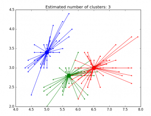
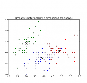
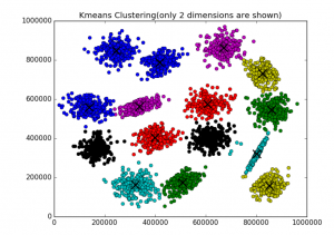
K-means Clustering Algorithm – is well known algorithm as the idea of this algorithm goes back to 1957. [2] The algorithm requires to input number of clusters and data. k-means clustering aims to partition n observations into k clusters in which each observation belongs to the cluster with the nearest mean.[2]. Below are shown results of K-means clustering of Iris dataset (only 2 dimensions shown) and clustering result for S1 dataset (see dataset section for more details).

k-means clustering Iris dataset

Fig 1. K-means clustering of Iris dataset


Fig 2. K-means clustering of S1 dataset

Affinity Propagation – performs affinity propagation clustering of data. In statistics and data mining, affinity propagation (AP) is a clustering algorithm based on the concept of “message passing” between data points. Unlike clustering algorithms such as k-means or k-medoids, affinity propagation does not require the number of clusters to be determined or estimated before running the algorithm. Similar to k-medoids, affinity propagation finds “exemplars”, members of the input set that are representative of clusters.[3]

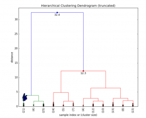
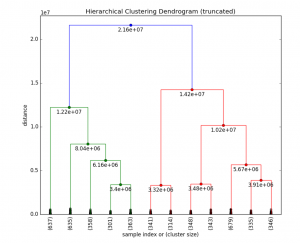
Hierarchical clustering (HC) – (also called hierarchical cluster analysis or HCA) is a method of cluster analysis which seeks to build a hierarchy of clusters. Strategies for hierarchical clustering generally fall into two types:

  • Agglomerative: This is a “bottom up” approach: each observation starts in its own cluster, and pairs of clusters are merged as one moves up the hierarchy.
  • Divisive: This is a “top down” approach: all observations start in one cluster, and splits are performed recursively as one moves down the hierarchy.

In general, the merges and splits are determined in a greedy manner. The results of hierarchical clustering are usually presented in a dendrogram. [4]

Birch algorithm – Back in the 1990s considerable effort has been put into improving the performance of existing algorithms. Among them is BIRCH (Zhang et al., 1996) [5]

BIRCH (balanced iterative reducing and clustering using hierarchies) is an unsupervised data mining algorithm used to perform hierarchical clustering over particularly large data-sets. An advantage of BIRCH is its ability to incrementally and dynamically cluster incoming, multi-dimensional metric data points in an attempt to produce the best quality clustering for a given set of resources (memory and time constraints). In most cases, BIRCH only requires a single scan of the database. [6]

Performance metrics for clustering algorithms

Silhouette refers to a method of interpretation and validation of consistency within clusters of data. The technique provides a succinct graphical representation of how well each object lies within its cluster. It was first described by Peter J. Rousseeuw in 1986.

The silhouette value is a measure of how similar an object is to its own cluster (cohesion) compared to other clusters (separation). The silhouette ranges from -1 to 1, where a high value indicates that the object is well matched to its own cluster and poorly matched to neighboring clusters. If most objects have a high value, then the clustering configuration is appropriate. If many points have a low or negative value, then the clustering configuration may have too many or too few clusters.
The silhouette can be calculated with any distance metric, such as the Euclidean distance or the Manhattan distance.[7]

Here is the python source code how to calculate the silhouette value for k-means clustering


from sklearn import cluster
from sklearn import metrics
import numpy as np


k=2
data = np.array([[1, 2],
              [5, 8],
              [1.5, 1.8],
              [8, 8],
              [1, 0.6],
              [9, 11]])


kmeans = cluster.KMeans(n_clusters=k)
kmeans.fit(data)


labels = kmeans.labels_
centroids = kmeans.cluster_centers_

print ("Cluster id labels for inputted data")
print (labels)
print ("Centroids data")
print (centroids)

print ("\nScore (Opposite of the value of X on the K-means objective which is Sum of distances of samples to their closest cluster center):")
print (kmeans.score(data))

silhouette_score = metrics.silhouette_score(data, labels, metric='euclidean')

print ("Silhouette_score: ")
print (silhouette_score)

Score (Opposite of the value of X on the K-means objective which is Sum of distances of samples to their closest cluster center) – Sum of distances of samples to their closest cluster center.

Large distances corresponds to a big variety in data samples and if the number of data samples is significantly higher than the number of clusters. On the contrary, if all data samples were the same, you would always get a zero distance regardless of number of clusters. [8]

Cophenetic correlation – In statistics, and especially in biostatistics, cophenetic correlation (more precisely, the cophenetic correlation coefficient) is a measure of how faithfully a dendrogram preserves the pairwise distances between the original unmodeled data points. Although it has been most widely applied in the field of biostatistics (typically to assess cluster-based models of DNA sequences, or other taxonomic models), it can also be used in other fields of inquiry where raw data tend to occur in clumps, or clusters. This coefficient has also been proposed for use as a test for nested clusters.[9]

Datasets
The following two datasets will be used:
The Iris flower data set or Fisher’s Iris data set is a multivariate data set – well know data set with N = 150 and k=3 [10] The data set consists of 50 samples from each of three species of Iris (Iris setosa, Iris virginica and Iris versicolor) [10]

S1 – Synthetic 2-d data with N=5000 vectors and k=15 Gaussian cluster [11]

Experiments
Using ML Sandbox tool and above clustering algorithms and datasets the clustering was performed. Screenshots of results of clustering from the tool were collected and presented here (Fig 1-6, Fig 1,2 are shown above)


Fig 3. AP clustering of Iris dataset


Fig 4. AP clustering results of Iris dataset


Fig 5. HC Clustering Iris dataset


Fig 6. HC clustering S1 dataset

Below in the summary of the above clustering experiments.

Kmeans (sklearn.cluster) AP (sklearn.cluster) HC (scipy.cluster) Birch (sklearn.cluster)
Score (Opposite of Sum of distances of samples to their closest cluster center) Silhouette_score Silhouette_score Cophenetic Correlation Coefficient: Silhouette_score
Iris dataset, 150, D4 -78.85 0.55 0.52 0.87 0.50
S1 dataset, 5000, D2 -8.92e+12 0.71 * 0.69 0.71

*AP did not work well on S1 dataset (but worked well on iris dataset) however there are some other optional parameters that can be used to resolve this. Probably need to be adjust preference parameter. Currently the tool does not allow change it.

From documentation [12] Preference is parameter that can be array-like, shape (n_samples,) or float, and is optional. Preferences for each point – points with larger values of preferences are more likely to be chosen as exemplars. The number of exemplars, ie of clusters, is influenced by the input preferences value. If the preferences are not passed as arguments, they will be set to the median of the input similarities.

ML Sandbox
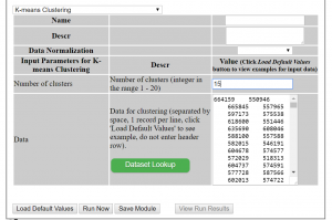
The above tool was used for clustering data. You need just select algorithm, enter your data and click run. Below are detailed instructions for clustering.
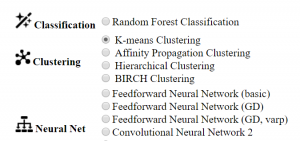
How to use the ML Sandbox
1. Open URL: ML Sandbox
2. Select Clustering method

3. Enter data (you can use default small dataset or copy and paste your dataset or dataset from other sites like iris, S1 see links in the references section)
4. Click Run Now

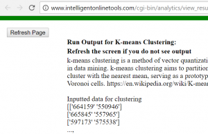
5. Click View Run Results
6. If you do not see results, click refresh button at top left corner. Depending on data set and algorithm you might need wait for a minute or two and click refresh.

Conclusion
We looked at different clustering methods, metrics performance and visualization of clustering results for different datasets. All of this can be done within online tool ML Sandbox Feel free to play with this tool and your data to explore your datasets. Also feel free to provide any feedback or suggestions.

References
1. Hierarchical Clustering: A Simple Explanation
2. k-means clustering
3. Affinity_propagation
4. Hierarchical clustering
5. Cluster_analysis
6. BIRCH
7. Silhouette (clustering)
8. understanding-score-returned-by-scikit-learn-kmeans
9. Cophenetic correlation
10. Iris flower data set
11. Clustering benchmark datasets
12 AffinityPropagation


Time Series Prediction with Convolutional Neural Networks and Keras

A convolutional neural network (CNNs) is a type of network that has recently
gained popularity due to its success in classification problems (e.g. image recognition
or time series classification) [1]. One of the working examples how to use Keras CNN for time series can be found at this link[2]. This example allows to predict for single time series and multivariate time series.

Running the code from this link, it was noticed that sometimes the prediction error has very high value, may be because optimizer gets stuck in local minimum. (See Fig1. The error is on axis Y and is very high for run 6) So I updated the script to run several times and then remove results with high error. (See Fig2 The Y axis showing small error values). Here is the summary of all changes:

  • Created multiple runs that can allow to filter bad results based on error. Training CNN is running 10 times and for each run error data and some other associated data is saved. Error is calculated as square root of sum if squared errors for last 10 predictions during the training.
  • Added also plot to see error over multiple runs.
  • In the end of script added one plot that showing errors for each run (See Fig1.) , and another plot showing errors only for runs that did not have high error (See Fig2.).
  • Added saving keras model to file for each run and then loading it from file for model that showed best results (min error). See [3] for more information on saving and loading keras models.
  • Added ability to load time series from csv file.

Error for all runs
Error for all runs
Fig 1.

Error chart after removing runs with high value error
Fig 2.

Below is the full code


#!/usr/bin/env python
"""
This code is based on convolutional neural network model from below link
gist.github.com/jkleint/1d878d0401b28b281eb75016ed29f2ee
"""

from __future__ import print_function, division

import numpy as np
from keras.layers import Convolution1D, Dense, MaxPooling1D, Flatten
from keras.models import Sequential
from keras.models import model_from_json

import matplotlib.pyplot as plt
import csv

__date__ = '2017-06-22'

error_total =[]
result=[]
i=0

def make_timeseries_regressor(window_size, filter_length, nb_input_series=1, nb_outputs=1, nb_filter=4):
    """:Return: a Keras Model for predicting the next value in a timeseries given a fixed-size lookback window of previous values.

    The model can handle multiple input timeseries (`nb_input_series`) and multiple prediction targets (`nb_outputs`).

    :param int window_size: The number of previous timeseries values to use as input features.  Also called lag or lookback.
    :param int nb_input_series: The number of input timeseries; 1 for a single timeseries.
      The `X` input to ``fit()`` should be an array of shape ``(n_instances, window_size, nb_input_series)``; each instance is
      a 2D array of shape ``(window_size, nb_input_series)``.  For example, for `window_size` = 3 and `nb_input_series` = 1 (a
      single timeseries), one instance could be ``[[0], [1], [2]]``. See ``make_timeseries_instances()``.
    :param int nb_outputs: The output dimension, often equal to the number of inputs.
      For each input instance (array with shape ``(window_size, nb_input_series)``), the output is a vector of size `nb_outputs`,
      usually the value(s) predicted to come after the last value in that input instance, i.e., the next value
      in the sequence. The `y` input to ``fit()`` should be an array of shape ``(n_instances, nb_outputs)``.
    :param int filter_length: the size (along the `window_size` dimension) of the sliding window that gets convolved with
      each position along each instance. The difference between 1D and 2D convolution is that a 1D filter's "height" is fixed
      to the number of input timeseries (its "width" being `filter_length`), and it can only slide along the window
      dimension.  This is useful as generally the input timeseries have no spatial/ordinal relationship, so it's not
      meaningful to look for patterns that are invariant with respect to subsets of the timeseries.
    :param int nb_filter: The number of different filters to learn (roughly, input patterns to recognize).
    """
    model = Sequential((
        # The first conv layer learns `nb_filter` filters (aka kernels), each of size ``(filter_length, nb_input_series)``.
        # Its output will have shape (None, window_size - filter_length + 1, nb_filter), i.e., for each position in
        # the input timeseries, the activation of each filter at that position.
        Convolution1D(nb_filter=nb_filter, filter_length=filter_length, activation='relu', input_shape=(window_size, nb_input_series)),
        MaxPooling1D(),     # Downsample the output of convolution by 2X.
        Convolution1D(nb_filter=nb_filter, filter_length=filter_length, activation='relu'),
        MaxPooling1D(),
        Flatten(),
        Dense(nb_outputs, activation='linear'),     # For binary classification, change the activation to 'sigmoid'
    ))
    model.compile(loss='mse', optimizer='adam', metrics=['mae'])
    # To perform (binary) classification instead:
    # model.compile(loss='binary_crossentropy', optimizer='adam', metrics=['binary_accuracy'])
    return model


def make_timeseries_instances(timeseries, window_size):
    """Make input features and prediction targets from a `timeseries` for use in machine learning.

    :return: A tuple of `(X, y, q)`.  `X` are the inputs to a predictor, a 3D ndarray with shape
      ``(timeseries.shape[0] - window_size, window_size, timeseries.shape[1] or 1)``.  For each row of `X`, the
      corresponding row of `y` is the next value in the timeseries.  The `q` or query is the last instance, what you would use
      to predict a hypothetical next (unprovided) value in the `timeseries`.
    :param ndarray timeseries: Either a simple vector, or a matrix of shape ``(timestep, series_num)``, i.e., time is axis 0 (the
      row) and the series is axis 1 (the column).
    :param int window_size: The number of samples to use as input prediction features (also called the lag or lookback).
    """
    timeseries = np.asarray(timeseries)
    assert 0 < window_size < timeseries.shape[0]
    X = np.atleast_3d(np.array([timeseries[start:start + window_size] for start in range(0, timeseries.shape[0] - window_size)]))
    y = timeseries[window_size:]
    q = np.atleast_3d([timeseries[-window_size:]])
    return X, y, q


def evaluate_timeseries(timeseries, window_size):
    """Create a 1D CNN regressor to predict the next value in a `timeseries` using the preceding `window_size` elements
    as input features and evaluate its performance.

    :param ndarray timeseries: Timeseries data with time increasing down the rows (the leading dimension/axis).
    :param int window_size: The number of previous timeseries values to use to predict the next.
    """
    filter_length = 5
    nb_filter = 4
    timeseries = np.atleast_2d(timeseries)
    if timeseries.shape[0] == 1:
        timeseries = timeseries.T       # Convert 1D vectors to 2D column vectors

    nb_samples, nb_series = timeseries.shape
    print('\n\nTimeseries ({} samples by {} series):\n'.format(nb_samples, nb_series), timeseries)
    model = make_timeseries_regressor(window_size=window_size, filter_length=filter_length, nb_input_series=nb_series, nb_outputs=nb_series, nb_filter=nb_filter)
    print('\n\nModel with input size {}, output size {}, {} conv filters of length {}'.format(model.input_shape, model.output_shape, nb_filter, filter_length))
    model.summary()

    error=[]
    
    X, y, q = make_timeseries_instances(timeseries, window_size)
    print('\n\nInput features:', X, '\n\nOutput labels:', y, '\n\nQuery vector:', q, sep='\n')
    test_size = int(0.01 * nb_samples)           # In real life you'd want to use 0.2 - 0.5
    X_train, X_test, y_train, y_test = X[:-test_size], X[-test_size:], y[:-test_size], y[-test_size:]
    model.fit(X_train, y_train, nb_epoch=25, batch_size=2, validation_data=(X_test, y_test))

    # serialize model to JSON
    model_json = model.to_json()
    with open("model"+str(i)+".json", "w") as json_file:
          json_file.write(model_json)
    # serialize weights to HDF5
    model.save_weights("model"+str(i)+".h5")
    print("Saved model to disk")
    global i
    i=i+1

    pred = model.predict(X_test)
    print('\n\nactual', 'predicted', sep='\t')
    error_curr=0
    for actual, predicted in zip(y_test, pred.squeeze()):
        print(actual.squeeze(), predicted, sep='\t')
        tmp = actual-predicted
        sum_squared = np.dot(tmp.T , tmp)
        error.append ( np.sqrt(sum_squared) )
        error_curr=error_curr+ np.sqrt(sum_squared)
    print('next', model.predict(q).squeeze(), sep='\t')
    result.append  (model.predict(q).squeeze())
    error_total.append (error_curr)
    print (error)

def read_file(fn):
    '''
    Reads the CSV file 
    -----
    RETURNS:
        A matrix with the file contents
    '''

    vals = []
    with open(fn, 'r') as csvfile:
        tsdata = csv.reader(csvfile, delimiter=',')
        for row in tsdata:
             vals.append(row) 

    # removing title row
    vals = vals[1:]
    y = np.array(vals).astype(np.float) 
    return y


def main():
    """Prepare input data, build model, eval uate."""
    np.set_printoptions(threshold=25)
    ts_length = 1000
    window_size = 50
    number_of_runs=10
    error_max=200
    
    print('\nSimple single timeseries vector prediction')
    timeseries = np.arange(ts_length)                   # The timeseries f(t) = t
    # enable below line to run this time series
    #evaluate_timeseries(timeseries, window_size)

    print('\nMultiple-input, multiple-output prediction')
    timeseries = np.array([np.arange(ts_length), -np.arange(ts_length)]).T      # The timeseries f(t) = [t, -t]
    # enable below line to run this time series
    ##evaluate_timeseries(timeseries, window_size)

    print('\nMultiple-input, multiple-output prediction')
    timeseries = np.array([np.arange(ts_length), -np.arange(ts_length), 2000-np.arange(ts_length)]).T      # The timeseries f(t) = [t, -t]
    # enable below line to run this time series
    #evaluate_timeseries(timeseries, window_size)
    
    timeseries = read_file('ts_input.csv')
    print (timeseries)
    
    for i in range(number_of_runs):
        evaluate_timeseries(timeseries, window_size)
        
    error_total_new=[]    
    for i in range(number_of_runs):
        if (error_total[i] < error_max):  
            error_total_new.append (error_total[i])
    
    plt.plot(error_total)
    plt.show()
    print (result)
    
    plt.plot(error_total_new)
    plt.show()
    print (result)
    
    best_model=np.asarray(error_total).argmin(axis=0)
    print ("best_model="+str(best_model))


    json_file = open('model'+str(best_model)+'.json', 'r')
    loaded_model_json = json_file.read()
    json_file.close()
    loaded_model = model_from_json(loaded_model_json)
    
    
    # load weights into new model
    loaded_model.load_weights("model"+str(best_model)+".h5")
    print("Loaded model from disk")


if __name__ == '__main__':
    main()

References
1. Conditional Time Series Forecasting with Convolutional Neural Networks
2. Example of using Keras to implement a 1D convolutional neural network (CNN) for timeseries prediction
3. Save and Load Your Keras Deep Learning Models


Forecasting Time Series Data with Convolutional Neural Networks

Convolutional neural networks(CNN) is increasingly important concept in computer science and finds more and more applications in different fields. Many posts on the web are about applying convolutional neural networks for image classification as CNN is very useful type of neural networks for image classification. But convolutional neural networks can also be used for applications other than images, such as time series prediction. This post is reviewing existing papers and web resources about applying CNN for forecasting time series data. Some resources also contain python source code.

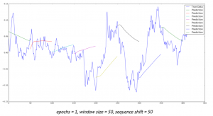
Deep neural networks opened new opportunities for time series prediction. New types of neural networks such as LSTM (variant of the RNN), CNN were applied for time series forecasting. For example here is the link for predicting time series with LSTM. [1] You can find here also the code. The code provides nice graph with ability to compare actual data and predicted data. (See figure below, sourced from [1]) Predictions start at different points of time so you can see and compare performance for several predictions.

Time series with LSTM

Below review is showing different approaches that can be used for forecasting time series data with convolutional neural networks.

1. Raw Data
The simplest way to feed data into neural network is to use raw data. Here is the link [2] to results of experiments with different types of neural networks including CNN. In this study stock data such as Date,Open,High,Low,Close,Volume,Adj Close were used with 3 types of networks: MLP, CNN and RNN.

CNN architecture was used as 2-layer convolutional neural network (combination of convolution and max-pooling layers) with one fully-connected layer. To improve performance the author suggests using different features (not only scaled time series) like some technical indicators, volume of sales.
According to [12] it is common to periodically insert a Pooling layer in-between successive Convolution layers in a CNN architecture. Its function is to progressively reduce the spatial size of the representation to reduce the amount of parameters and computation in the network, and hence to also control overfitting. The Pooling Layer operates independently on every depth slice of the input and resizes it spatially, using the MAX operation.

2. Automatic Selection of Features
Transforming data before inputting to neural network is common practice. We can use feature based methods like described here in Feature-selection-time-series-forecasting-python or filtering methods like removing trend, seasonality or low pass / high pass filtering.
With deep learning it is possible to lean features automatically. For example in one research the authors introduce a deep learning framework for multivariate time series classification: Multi-Channels Deep Convolutional Neural Networks (MCDCNN). Multivariate time series are separated into univariate ones and perform feature learning on each univariate series individually. Then a
normal MLP is concatenated at the end of feature learning to do classification. [3]
The CNN architecture consists of 2 layer CNN (combination of filter, activation and pooling layers) and 2 Fully connected layers that represent classification MLP.

3. Fully Convolutional Neural Network (FCN)
In this study different neural network architectures such as Multilayer Perceptrons, Fully convolutional NN (FCN), Residual Network are proposed. For FCN authors build the final networks by stacking three convolution blocks with the filter sizes {128, 256, 128} in each block. Unlike the MCNN and MC-CNN, any pooling operation is excluded. This strategy helps to prevent overfitting. Batch normalization is applied to speed up the convergence speed and help improve generalization.

After the convolution blocks, the features are fed into a global average pooling layer instead of a fully connected layer, which largely reduces the number of weights. The final label is produced by a softmax layer. [4] Thus the architecture of neural network consists of three convolution blocks and global average pooling and softmax layers in the end.

4. Different Data Transformations
In this study [5] CNNs were trained with different data transformations, which included: the entire dataset, spatial clustering, and PCA decomposition. Data was also fit to the hidden modules of a Clockwork Recurrent Neural Network. This type of recurrent network (CRNN) has the advantage of maintaining a high-temporal-resolution memory in its hidden layers after training.

This network also overcomes the problem of the vanishing gradient found in other RNNs by partitioning the neurons in its hidden layers as different ”sub-clocks” that are able to capture the input to the network at different time steps. Here you can find more about CRNN [11]. According to this paper a clockwork RNN architecture is similar to a simple RNN with an input, output and hidden layer. The hidden layer is partitioned into g modules each with its own clock rate. Within each module the neurons are fully interconnected.

5. Analysing Multiple Time Series Relationships
This paper [6] focuses on analyzing multiple time series relationships such as correlations between them. Authors show that deep learning methods for time series processing are comparable to the other approaches and have wide opportunities for further improvement. Range of methods is discussed and code optimisations is applied for the convolutional neural network for the forecasting time series data domain.

6. Data Augmentation
In this study two approaches are proposed to artificially increase the size of training sets. The first one is based on data-augmentation techniques. The second one consists in mixing different training sets and learning the network in a semi-supervised way. The authors show that these two approaches improve the overall classification performance.

7. Encoding data as image
Another methodology for time series with convolutional neural networks that got popular with deep learning is encoding data as the image. Here data is encoded as images which feed to neural network. This enables the use of techniques from computer vision for classification.
Here [8] is the link where python script can be found for encoding data as image. It encodes data into formats such as GAF, MTF. The script has the dependencies on python modules such as Numpy, Pandas, Matplolib and Cpickle.

Theory of using image encoded data is described in [9]. In this paper a novel framework proposes to encode time series data as different types of images, namely, Gramian Angular Fields (GAF) and Markov Transition Fields (MTF).

Learning Traffic as Images:
This paper [10] proposes a convolutional neural network (CNN)-based method that learns traffic as images and predicts large-scale, network-wide traffic speed with a high accuracy. Spatiotemporal traffic dynamics are converted to images describing the time and space relations of traffic flow via a two-dimensional time-space matrix. A CNN is applied to the image following two consecutive steps: abstract traffic feature extraction and network-wide traffic speed prediction. CNN architecture consists of several convolutional and pooling layers and fully connected layer in the end for prediction.

Conclusion

Deep learning and convolutional neural networks created new opportunities for forecasting time series data domain. The above text presents different techniques that can be used in time series prediction with convolutional neural networks. The common part that we can see in most of studies is that feature extraction can be done via deep learning automatically in CNN or in other words, CNNs can learn features on their own. Below you can see architecture of CNN at very high level. The actual implementations can vary in different ways, some of them were shown above.

CNN Architecture for Forecasting Time Series Data

References

1. LSTM NEURAL NETWORK FOR TIME SERIES PREDICTION
2. Neural networks for algorithmic trading. Part One — Simple time series forecasting
3. Time Series Classification Using Multi-Channels Deep Convolutional Neural Networks
4. Time Series Classification from Scratch with Deep Neural Networks: A Strong Baseline
5. Assessing Neuroplasticity with Convolutional and Recurrent Neural Networks
6. Signal Correlation Prediction Using Convolutional Neural Networks
7. Data Augmentation for Time Series Classification using Convolutional Neural Networks.
8. Imaging-time-series-to-improve-classification-and-imputation
9. Encoding Time Series as Images for Visual Inspection and Classification Using
Tiled Convolutional Neural Networks

10. Learning Traffic as Images: A Deep Convolutional Neural Network for Large-Scale Transportation Network Speed Prediction
11. A Clockwork RNN
12. CS231n Convolutional Neural Networks for Visual Recognition