Time Series Analysis with Python and Prophet

Recently Facebook released Prophet – open source software tool for forecasting time series data.
Facebook team have implemented in Prophet two trend models that can cover many applications: a saturating growth model, and a piecewise linear model. [4]

With growth model Prophet can be used for prediction growth/decay – for example for modeling growth of population or website traffic. By default, Prophet uses a linear model for its forecast.

In this post we review main features of Prophet and will test it on prediction of stock data prices for next 10 business days. We will use python for time series programming with Prophet.

How to Use Prophet for Time Series Analysis with Python

Here is the minimal python source code to create forecast with Prophet.

import pandas as pd
from fbprophet import Prophet

The input columns should have headers as ‘ds’ and ‘y’. In the code below we run forecast for 180 days ahead for stock data, ds is our date stamp data column, and y is actual time series column

fname="C:\\Users\\data analysis\\gm.csv"
data = pd.read_csv (fname)

data.columns = ['ds', 'y']
model = Prophet() 
model.fit(data); #fit the model
future_stock_data = model.make_future_dataframe(periods=180, freq = 'd')
forecast_data = model.predict(future_stock_data)
print ("Forecast data")
model.plot(forecast_data)

The result of the above code will be graph shown below.

time series analysis python using Prophet

Time series model consists of three main model components: trend, seasonality, and holidays.
We can print components using the following line

model.plot_components(forecast_data)
time series analysis python - components
time series analysis python – components

Can Prophet be Used for Data Stock Price Prediction?

It is interesting to know if Prophet can be use for financial market price forecasting. The practical question is how accurate forecasting with Prophet for stock data prices? Data analytics for stock market is known as hard problem as many different events influence stock prices every day. To check how it works I made forecast for 10 days ahead using actual stock data and then compared Prophet forecast with actual data.

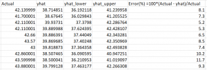
The error was calculated for each day for data stock price (closed price) and is shown below

Data stock price prediction analysis

Based on obtained results the average error is 7.9% ( this is 92% accuracy). In other words the accuracy is sort of low for stock prices prediction. But note that all errors have the same sign. May be Prophet can be used better for prediction stock market direction? This was already mentioned in another blog [2].
And also looks like the error is not changing much with the the time horizon, at least within first 10 steps. Forecasts for days 3,4,5 even have smaller error than for the day 1 and 2.

Further looking at more data would be interesting and will follow soon. Bellow is the full python source code.


import pandas as pd
from fbprophet import Prophet


fname="C:\\Users\\GM.csv"
data = pd.read_csv (fname)
data.columns = ['ds', 'y']
model = Prophet() #instantiate Prophet
model.fit(data); #fit the model with your dataframe

future_stock_data = model.make_future_dataframe(periods=10, freq = 'd')
forecast_data = model.predict(future_stock_data)

print ("Forecast data")
print (forecast_data[['ds', 'yhat', 'yhat_lower', 'yhat_upper']].tail(12))
	
model.plot(forecast_data)
model.plot_components(forecast_data)

References
1. Stock market forecasting with prophet
2. Can we predict stock prices with Prophet?
3. Saturating Forecasts
4. Forecasting at Scale


Regression and Classification Decision Trees – Building with Python and Running Online

According to survey [1] Decision Trees constitute one of the 10 most popular data mining algorithms.
Decision trees used in data mining are of two main types:
Classification tree analysis is when the predicted outcome is the class to which the data belongs.
Regression tree analysis is when the predicted outcome can be considered a real number (e.g. the price of a house, or a patient’s length of stay in a hospital).[2]

In the previous posts I already covered how to create Regression Decision Trees with python:

Building Decision Trees in Python
Building Decision Trees in Python – Handling Categorical Data

In this post you will find more simplified python code for classification and regression decision trees. Online link to run decision tree also will be provided. This is very useful if you want see results immediately without coding.

To run the code provided here you need just change file path to file containing data. The Decision Trees in this post are tested on simple artificial dataset that was motivated by doing feature selection for blog data:

Getting Data-Driven Insights from Blog Data Analysis with Feature Selection

Dataset
Our dataset consists of 3 columns in csv file and shown below. It has 2 independent variables (features or X columns) – categorical and numerical, and dependent numerical variable (target or Y column). The script is assuming that the target column is the last column. Below is the dataset that is used in this post:


X1	X2	Y
red	1	100
red	2	99
red	1	85
red	2	100
red	1	79
red	2	100
red	1	100
red	1	85
red	2	100
red	1	79
blue	2	22
blue	1	20
blue	2	21
blue	1	13
blue	2	10
blue	1	22
blue	2	20
blue	1	21
blue	2	13
blue	1	10
blue	1	22
blue	2	20
blue	1	21
blue	2	13
blue	1	10
blue	2	22
blue	1	20
blue	2	21
blue	1	13
green	2	10
green	1	22
green	2	20
green	1	21
green	2	13
green	1	10
green	2	22
green	1	20
green	1	13
green	2	22
green	1	20
green	2	21
green	1	13
green	2	10

You can use dataset with different number of columns for independent variables without changing the code.

For converting categorical variable to numerical we use here pd.get_dummies(dataframe) method from pandas library. Here dataframe is our input data. So the column with “green”, “red”, “yellow” will be transformed in 3 columns with 0,1 values in each (one hot encoding scheme). Below are the few first rows after converting:


N   X2  X1_blue  X1_green  X1_red    Y
0    1      0.0       0.0     1.0  100
1    2      0.0       0.0     1.0   99
2    1      0.0       0.0     1.0   85
3    2      0.0       0.0     1.0  100

Python Code
Two scripts are provided here – regressor and classifier. For classifier the target variable should be categorical. We use however same dataset but convert numerical continuous variable to classes with labels (A,B,C) within the script based on inputted bin ranges ([15,50,100] which means bins 0-15, 15.001-50, 50.001-100). We use this after applying get_dummies

What if you have categorical target? Calling get_dummies will convert it to numerical too but we do not want this. In this case you need specify explicitly what columns need to be converted via parameter columns As per the documentation:
columns : list-like, default None. This is column names in the DataFrame to be encoded. If columns is None then all the columns with object or category dtype will be converted. [3]
In our example we would need to do specify column X1 like this:
dataframe=pd.get_dummies(dataframe, columns=[“X1”])

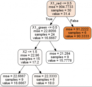
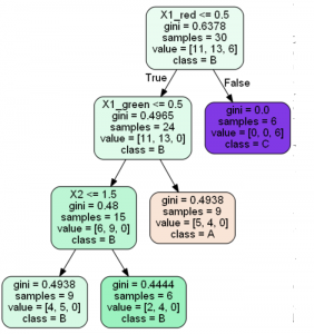
The results of running scripts are decision trees shown below:
Decision Tree Regression
Decision Tree Classification
Running Decision Trees Online
In case you do not want to play with python code, you can run Decision Tree algorithms online at ML Sandbox
All that you need is just enter data into the data fields, here are the instructions:

  1. Go to ML Sandbox
  2. Select Decision Classifier OR Decision Regressor
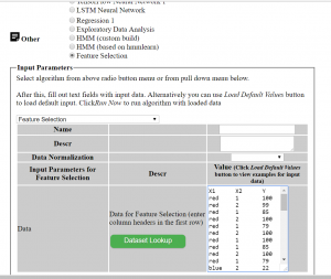
  3. Enter data (first row should have headers) OR click “Load Default Values” to load the example data from this post. See screenshot below
  4. Click “Run Now“.
  5. Click “View Run Results
  6. If you do not see yet data wait for a minute or so and click “Refresh Page” and you will see results
  7. Note: your dependent variable (target variable or Y variable) should be in most right column. Also do not use space in the words (header and data)

    Conclusion
    Decision Trees belong to the top 10 machine learning or data mining algorithms and in this post we looked how to build Decision Trees with python. The source code provided is the end of this post. We looked also how do this if one or more columns are categorical. The source code was tested on simple categorical and numerical example and provided in this post. Alternatively you can run same algorithm online at ML Sandbox

    References

    1. Top 10 Machine Learning Algorithms for Beginners
    2. Decision Tree Learning
    3. pandas.get_dummies

    Here is the python computer code of the scripts.
    DecisionTreeRegressor

    
    # -*- coding: utf-8 -*python computer code-
    
    import pandas as pd
    from sklearn.cross_validation import train_test_split
    from sklearn.tree import DecisionTreeRegressor
    
    
    import subprocess
    
    from sklearn.tree import  export_graphviz
    
    
    def visualize_tree(tree, feature_names):
        
        with open("dt.dot", 'w') as f:
            
            export_graphviz(tree, out_file=f, feature_names=feature_names,  filled=True, rounded=True )
    
        command = ["C:\\Program Files (x86)\\Graphviz2.38\\bin\\dot.exe", "-Tpng", "C:\\Users\\Owner\\Desktop\\A\\Python_2016_A\\dt.dot", "-o", "dt.png"]
        
            
        try:
            subprocess.check_call(command)
        except:
            exit("Could not run dot, ie graphviz, to "
                 "produce visualization")


    filename = "C:\\Users\\Owner\\Desktop\\A\\Blog Analytics\\data1.csv"
    dataframe = pd.read_csv(filename, sep= ',' )


    cols = dataframe.columns.tolist()
    last_col_header = cols[-1]
    
    
    dataframe=pd.get_dummies(dataframe)
    cols = dataframe.columns.tolist()
    
    cols.insert(len(dataframe.columns)-1, cols.pop(cols.index(last_col_header)))
    dataframe = dataframe.reindex(columns= cols)
    
    print (dataframe)


    array = dataframe.values
    X = array[:,0:len(dataframe.columns)-1]  
    Y = array[:,len(dataframe.columns)-1]   
    print ("--X----")
    print (X)
    print ("--Y----")
    print (Y)
    
                           
    X_train, X_test, y_train, y_test = train_test_split( X, Y, test_size = 0.3, random_state = 100)                           
                               
    clf = DecisionTreeRegressor( random_state = 100,
                                   max_depth=3, min_samples_leaf=4)
    clf.fit(X_train, y_train)   
    
    visualize_tree(clf, dataframe.columns)
    

    DecisionTreeClassifier

    
    # -*- coding: utf-8 -*-
    
    import pandas as pd
    from sklearn.cross_validation import train_test_split
    from sklearn.tree import DecisionTreeClassifier
    
    import subprocess
    
    from sklearn.tree import  export_graphviz
    
    
    def visualize_tree(tree, feature_names, class_names):
        
        with open("dt.dot", 'w') as f:
            
            export_graphviz(tree, out_file=f, feature_names=feature_names,  filled=True, rounded=True, class_names=class_names )
    
        command = ["C:\\Program Files (x86)\\Graphviz2.38\\bin\\dot.exe", "-Tpng", "C:\\Users\\Owner\\Desktop\\A\\Python_2016_A\\dt.dot", "-o", "dt.png"]
        
            
        try:
            subprocess.check_call(command)
        except:
            exit("Could not run dot, ie graphviz, to "
                 "produce visualization")


    values=[15,50,100]
    def convert_to_label (a):
        count=0
        for v in values:
            if (a <= v) :
                return chr(ord('A') + count)
            else:
                count=count+1
        
        
    filename = "C:\\Users\\Owner\\Desktop\\A\\Blog Analytics\\data1.csv"
    dataframe = pd.read_csv(filename, sep= ',' )
    
    cols = dataframe.columns.tolist()
    last_col_header = cols[-1]
    dataframe=pd.get_dummies(dataframe)
    cols = dataframe.columns.tolist()
    
    
    print (dataframe)
    
    
    for index, row in dataframe.iterrows():
           dataframe.loc[index, "Y"] = convert_to_label(dataframe.loc[index, "Y"])


    cols.insert(len(dataframe.columns)-1, cols.pop(cols.index('Y')))
    dataframe = dataframe.reindex(columns= cols)
    
    print (dataframe)
    
    array = dataframe.values
    X = array[:,0:len(dataframe.columns)-1]  
    Y = array[:,len(dataframe.columns)-1]   
    print ("--X----")
    print (X)
    print ("--Y----")
    print (Y)
                           
    X_train, X_test, y_train, y_test = train_test_split( X, Y, test_size = 0.3, random_state = 100)                           
                               
    
    clf = DecisionTreeClassifier(criterion = "gini", random_state = 100,
                                   max_depth=3, min_samples_leaf=4)
    
    
    clf.fit(X_train, y_train)   
    
    clm=dataframe[last_col_header]
    clmvalues = clm.unique()
    visualize_tree(clf, dataframe.columns, clmvalues )


Getting Data-Driven Insights from Blog Data Analysis with Feature Selection

Machine learning algorithms are widely used in every business – object recognition, marketing analytics, analyzing data in numerous applications to get useful insights. In this post one of machine learning techniques is applied to analysis of blog post data to predict significant features for key metrics such as page views.

You will see in this post simple example that will help to understand how to use feature selection with python code. Instructions how to quickly run online feature selection algorithm will be provided also. (no sign up is needed)

Feature Selection
In machine learning and statistics, feature selection, also known as variable selection, attribute selection or variable subset selection, is the process of selecting a subset of relevant features (variables, predictors) for use in model construction.[1]. Using feature selection we can identify most influential variables for our metrics.

The Problem – Blog Data and the Goal
For example for each post you can have the following independent variables, denoted usually X

  1. Number of words in the post
  2. Post Category (or group or topic)
  3. Type of post (for example: list of resources, description of algorithms )
  4. Year when the post was published

The list can go on.
Also for each posts there are some metrics data or dependent variables denoted by Y. Below is an example:

  1. Number of views
  2. Times on page
  3. Revenue $ amount associated with the page view

The goal is to identify how X impacts on Y or predict Y based on X. Knowing most significant X can provide insights on what actions need to be taken to improve Y.
In this post we will use feature selection from python ski-learn library. This technique allows to rank the features based on their influence on Y.

Example with Simple Dataset
First let’s look at artificial dataset below. It is small and only has few columns so you can see some correlation between X and Y even without running algorithm. This allows us to test the results of algorithm to confirm that it is running correctly.


X1	X2	Y
red	1	100
red	2	99
red	1	85
red	2	100
red	1	79
red	2	100
red	1	100
red	1	85
red	2	100
red	1	79
blue	2	22
blue	1	20
blue	2	21
blue	1	13
blue	2	10
blue	1	22
blue	2	20
blue	1	21
blue	2	13
blue	1	10
blue	1	22
blue	2	20
blue	1	21
blue	2	13
blue	1	10
blue	2	22
blue	1	20
blue	2	21
blue	1	13
green	2	10
green	1	22
green	2	20
green	1	21
green	2	13
green	1	10
green	2	22
green	1	20
green	1	13
green	2	22
green	1	20
green	2	21
green	1	13
green	2	10

Categorical Data
You can see from the above data that our example has categorical data (column X1) which require special treatment when we use ski-learn library. Fortunately we have function get_dummies(dataframe) that converts categorical variables to numerical using one hot encoding. After convertion instead of one column with blue, green and red we will get 3 columns with 0,1 for each color. Below is the dataset with new columns:


N   X2  X1_blue  X1_green  X1_red    Y
0    1      0.0       0.0     1.0  100
1    2      0.0       0.0     1.0   99
2    1      0.0       0.0     1.0   85
3    2      0.0       0.0     1.0  100
4    1      0.0       0.0     1.0   79
5    2      0.0       0.0     1.0  100
6    1      0.0       0.0     1.0  100
7    1      0.0       0.0     1.0   85
8    2      0.0       0.0     1.0  100
9    1      0.0       0.0     1.0   79
10   2      1.0       0.0     0.0   22
11   1      1.0       0.0     0.0   20
12   2      1.0       0.0     0.0   21
13   1      1.0       0.0     0.0   13
14   2      1.0       0.0     0.0   10
15   1      1.0       0.0     0.0   22
16   2      1.0       0.0     0.0   20
17   1      1.0       0.0     0.0   21
18   2      1.0       0.0     0.0   13
19   1      1.0       0.0     0.0   10
20   1      1.0       0.0     0.0   22
21   2      1.0       0.0     0.0   20
22   1      1.0       0.0     0.0   21
23   2      1.0       0.0     0.0   13
24   1      1.0       0.0     0.0   10
25   2      1.0       0.0     0.0   22
26   1      1.0       0.0     0.0   20
27   2      1.0       0.0     0.0   21
28   1      1.0       0.0     0.0   13
29   2      0.0       1.0     0.0   10
30   1      0.0       1.0     0.0   22
31   2      0.0       1.0     0.0   20
32   1      0.0       1.0     0.0   21
33   2      0.0       1.0     0.0   13
34   1      0.0       1.0     0.0   10
35   2      0.0       1.0     0.0   22
36   1      0.0       1.0     0.0   20
37   1      0.0       1.0     0.0   13
38   2      0.0       1.0     0.0   22
39   1      0.0       1.0     0.0   20
40   2      0.0       1.0     0.0   21
41   1      0.0       1.0     0.0   13
42   2      0.0       1.0     0.0   10

If you run python script (provided in this post) you will get feature score like below.
Columns:
X2 X1_blue X1_green X1_red
scores:
[ 0.925 5.949 4.502 33. ]

So it is showing that column with red color is most significant and this makes sense if you look at data.

How to Run Script
To run script you need put data in csv file and update filename location in the script.
Additionally you need to have dependent variable Y in most right column and it should be labeled by ‘Y’.
The script is using option ‘all’ for number of features, but you can change some number if needed.

Example with Dataset from Blog
Now we can move to actual dataset from this blog. It took a little time to prepare data but this is just for the first time. Going forward I am planning to record data regularly after I create post or at least on weekly basis. Here are the fields that I used:

  1. Number of words in the post – this is something that the blog is providing
  2. Category or group or topic – was added manually
  3. Type of post – I used few groups for this
  4. Number of views – was taken from Google Analytics

For the first time I just used data from 19 top posts.

Results
Below you can view results. The results are showing word count as significant, which could be expected, however I would think that score should be less. The results show also higher score for posts with text and code vs the posts with mostly only code (Type_textcode 10.9 vs Type_code 5.0)

Feature Score
WordsCount 2541.55769
Group_DecisionTree 18
Group_datamining 18
Group_machinelearning 18
Group_spreadsheet 18
Group_TSCNN 17
Group_python 16
Group_TextMining 12.25
Type_textcode 10.88888889
Group_API 10.66666667
Group_Visualization 9.566666667
Group_neuralnetwork 5.333333333
Type_code 5.025641026

Running Online
In case you do not want to play with python code, you can run feature selection online at ML Sandbox
All that you need is just enter data into the data field, here are the instructions:

  1. Go to ML Sandbox
  2. Select Feature Extraction next Other
  3. Enter data (first row should have headers) OR click “Load Default Values” to load the example data from this post. See screenshot below
  4. Click “Run Now“.
  5. Click “View Run Results
  6. If you do not see yet data wait for a minute or so and click “Refresh Page” and you will see results
  7. Note: your dependent variable Y should be in most right column and should have header Y Also do not use space in the words (header and data)

    Conclusion
    In this post we looked how one of machine learning techniques – feature selection can be applied for analysis blog post data to predict significant features that can help choose better actions. We looked also how do this if one or more columns are categorical. The source code was tested on simple categorical and numerical example and provided in this post. Alternatively you can run same algorithm online at ML Sandbox

    Do you run any analysis on blog data? What method do you use and how do you pull data from blog? Feel free to submit any comments or suggestions.

    References
    1. Feature Selection Wikipedia
    2. Feature Selection For Machine Learning in Python

    
    # -*- coding: utf-8 -*-
    
    # Feature Extraction with Univariate Statistical Tests
    import pandas
    import numpy
    from sklearn.feature_selection import SelectKBest
    from sklearn.feature_selection import chi2
    
    
    filename = "C:\\Users\\Owner\\data.csv"
    dataframe = pandas.read_csv(filename)
    
    dataframe=pandas.get_dummies(dataframe)
    cols = dataframe.columns.tolist()
    cols.insert(len(dataframe.columns)-1, cols.pop(cols.index('Y')))
    dataframe = dataframe.reindex(columns= cols)
    
    print (dataframe)
    print (len(dataframe.columns))
    
    
    array = dataframe.values
    X = array[:,0:len(dataframe.columns)-1]  
    Y = array[:,len(dataframe.columns)-1]   
    print ("--X----")
    print (X)
    print ("--Y----")
    print (Y)
    # feature extraction
    test = SelectKBest(score_func=chi2, k="all")
    fit = test.fit(X, Y)
    # summarize scores
    numpy.set_printoptions(precision=3)
    print ("scores:")
    print(fit.scores_)
    
    for i in range (len(fit.scores_)):
        print ( str(dataframe.columns.values[i]) + "    " + str(fit.scores_[i]))
    features = fit.transform(X)
    
    print (list(dataframe))
    
    numpy.set_printoptions(threshold=numpy.inf)
    print ("features")
    print(features)


10 New Top Resources on Machine Learning from Around the Web

For this post I put new and most interesting machine learning resources that I recently found on the web. This is the list of useful resources in such areas like stock market forecasting, text mining, deep learning, neural networks and getting data from Twitter. Hope you enjoy the reading.

1. Stock market forecasting with prophet – this post belongs to series of posts about using Prophet which is the tool for producing high quality forecasts for time series data that has multiple seasonality with linear or non-linear growth. You will find here different techniques for stock data forecasting.
Prophet is open source software released by Facebook’s Core Data Science team. It is available for download on CRAN and PyPI.

2. Python For Finance: Algorithmic Trading – Another post about stock data analysis with python. This tutorial introduces you to algorithmic trading, and much more.

3. Recommendation and trend analysis is interesting topic. You can read this post to find out how to improve algorithms: recommendation-engine-for-trending-products-in-python In this post author is proposing new trending products algorithm in order to increase serendipity. This will allow to show to user something the user would not expect, but still could find interesting.

4. Word2Vec word embedding tutorial in Python and TensorFlow This tutorial is covering “Word2Vec” technique. This methodology is used in NLP to efficiently convert words into numeric vectors.

5. Best Practices for Document Classification with Deep Learning In this post you will find review of some best practices how to use deep learning for text classification. From the examples in this post you will discover different type of Convolutional Neural Networks (CNN) architecture.

6. How to Develop a Deep Learning Bag-of-Words Model for Predicting Movie Review Sentiment In this post you will find how to use deep learning model for sentiment analysis. The model is simple feedforward network with fully connected layers.

7. How to Clean Text for Machine Learning with Python – Here you will find great and complete tutorial for text preprocessing with python. Also links to resources for further learning are provided too.

8. Gathering Tweets with Python. This tutorial guides you in setting up a system for collecting Tweets.

9. Twitter Data Mining: A Guide To Big Data Analytics Using Python Here you can also find how to connect to Twitter and extract some tweets.

10. Stream data from Twitter using Python This post will show you how to get all identification information required for connecting to Twitter. Also you will find here how to receive tweets via the stream from Twitter.


Data Visualization of Word Correlations with NetworkX

This is a continuation of my previous post, found here Combining Machine Learning and Data Scraping. Data visualization is added to show correlations between words. The graph was built using NetworkX python library.
The input for the graph is the array corr_data with 3 columns : pair of words and correlation between them. This was calculated in the previous post.

In this post are added two functions:
build_graph_for_all – it is taking words from matrix for the first N rows and adding to the graph.
The graph is shown below.

The Second function build_graph is taking specific word and adding to graph only edge that have this word. The process is repeating but now it is adding edges to other words on the graph. This is recursive function. Below in the python code are shown these functions.

Python computer code:


import networkx as nx
import matplotlib.pyplot as plt
G=nx.Graph()

existing_edges = {}

def build_graph(w, lev):
  if (lev > 5)  :
      return
  for z in corr_data:
     ind=-1 
     if z[0] == w:
         ind=0
         ind1=1
     if z[1] == w:
         ind ==1
         ind1 =0
         
     if ind == 0 or ind == 1:
         if  str(w) + "_" + str(corr_data[ind1]) not in existing_edges :
            
             G.add_node(str(corr_data[ind]))
             existing_edges[str(w) + "_" + str(corr_data[ind1])] = 1;
             G.add_edge(w,str(corr_data[ind1]))
            
             build_graph(corr_data[ind1], lev+1)


existing_nodes = {}
def build_graph_for_all():
    count=0
    for d in corr_data:
        if (count > 40) :
            return
        if  d[0] not in existing_edges :
             G.add_node(str(d[0]))
        if  d[1] not in existing_edges :     
             G.add_node(str(d[1]))
        G.add_edge(str(d[0]), str(d[1]))     
        count=count + 1


build_graph_for_all()

print (G.nodes(data=True))
plt.show()
nx.draw(G, width=2, with_labels=True)
plt.savefig("path1.png")


w="design"
G.add_node(w)
build_graph(w, 0)
 
print (G.nodes(data=True))
plt.show()
nx.draw(G, width=2, with_labels=True)
plt.savefig("path.png")

In this post we created script that can be used to draw plot of connections between the words. In the near future I am planning to apply this technique to real problem. Below is the full source code.


# -*- coding: utf-8 -*-

import numpy as np
import nltk
import csv
import re
from scipy.stats.stats import pearsonr   

def remove_html_tags(text):
        """Remove html tags from a string"""
        clean = re.compile('<.*?>')
        return re.sub(clean, '', text)


fn="C:\\Users\\Owner\\Desktop\\A\\Scrapping\\craigslist\\result-jobs-multi-pages-content.csv"

docs=[]
def load_file(fn):
         start=1
         file_urls=[]
         
         strtext=""
         with open(fn, encoding="utf8" ) as f:
            csv_f = csv.reader(f)
            for i, row in enumerate(csv_f):
               if i >=  start  :
                 file_urls.append (row)
                
                 strtext=strtext + replaceNotNeeded(str(stripNonAlphaNum(row[5])))
                 docs.append (str(stripNonAlphaNum(row[5])))
                
         return strtext  
     

# Given a text string, remove all non-alphanumeric
# characters (using Unicode definition of alphanumeric).

def stripNonAlphaNum(text):
    import re
    return re.compile(r'\W+', re.UNICODE).split(text)

def replaceNotNeeded(text):
    text=text.replace("'","").replace(",","").replace ("''","").replace("'',","")
    text=text.replace(" and ", " ").replace (" to ", " ").replace(" a "," ").replace(" the "," ").replace(" of "," ").replace(" in "," ").replace(" for ", " ").replace(" or ", " ")
    text=text.replace(" will ", " ").replace (" on ", " ").replace(" be "," ").replace(" with "," ").replace(" is "," ").replace(" as "," ")
    text=text.replace("    "," ").replace("   "," ").replace("  "," ")
    return text

txt=load_file(fn)
print (txt)

tokens = nltk.wordpunct_tokenize(str(txt))

my_count = {}
for word in tokens:
    try: my_count[word] += 1
    except KeyError: my_count[word] = 1

print (my_count)


data = []

sortedItems = sorted(my_count , key=my_count.get , reverse = True)
item_count=0
for element in sortedItems :
       if (my_count.get(element) > 3):
           data.append([element, my_count.get(element)])
           item_count=item_count+1


N=5
topN = []
corr_data =[]
for z in range(N):
    topN.append (data[z][0])


wcount = [[0 for x in range(500)] for y in range(2000)] 
docNumber=0     
for doc in docs:
    
    for z in range(item_count):
        
        wcount[docNumber][z] = doc.count (data[z][0])
    docNumber=docNumber+1

print ("calc correlation")        
     
for ii in range(N-1):
    for z in range(item_count):
       
        r_row, p_value = pearsonr(np.array(wcount)[:, ii], np.array(wcount)[:, z])
        print (r_row, p_value)
        if r_row > 0.6 and r_row < 1:
               corr_data.append ([topN[ii],  data[z][0], r_row])
        
print ("correlation data")
print (corr_data)


import networkx as nx
import matplotlib.pyplot as plt
G=nx.Graph()

existing_edges = {}

def build_graph(w, lev):
  if (lev > 5)  :
      return
  for z in corr_data:
     ind=-1 
     if z[0] == w:
         ind=0
         ind1=1
     if z[1] == w:
         ind ==1
         ind1 =0
         
     if ind == 0 or ind == 1:
         if  str(w) + "_" + str(corr_data[ind1]) not in existing_edges :
            
             G.add_node(str(corr_data[ind]))
             existing_edges[str(w) + "_" + str(corr_data[ind1])] = 1;
             G.add_edge(w,str(corr_data[ind1]))
            
             build_graph(corr_data[ind1], lev+1)


existing_nodes = {}
def build_graph_for_all():
    count=0
    for d in corr_data:
        if (count > 40) :
            return
        if  d[0] not in existing_edges :
             G.add_node(str(d[0]))
        if  d[1] not in existing_edges :     
             G.add_node(str(d[1]))
        G.add_edge(str(d[0]), str(d[1]))     
        count=count + 1


build_graph_for_all()

print (G.nodes(data=True))
plt.show()
nx.draw(G, width=2, with_labels=True)
plt.savefig("path5.png")

w="design"

G.add_node(w)

build_graph(w, 10)

print (G.nodes(data=True))
plt.show()
nx.draw(G, width=2, with_labels=True)
plt.savefig("path.png")